Nonlinear finite elements/Homework 7/Solutions

< Nonlinear finite elements < Homework 7

Problem 1: Index Notation

Solutions

Part 1

Determine whether the following expressions are valid in index notation. If valid, identify the free indices and the dummy indices.

1) $A_{ms} = b_m (c_r - d_r)$

Invalid. The free indices are $m,s$ on the LHS and $m,r$ on the RHS.

2) $A_{ms} = b_m (c_s - d_s)$

Valid. Both $m$ and $s$ are free indices.

3) $t_i= \sigma_{ji} n_j$

Valid. The free index is $i$ and the dummy index is $j$ .

4) $t_i= \sigma_{ji} n_i$

Invalid. The free index is $i$ on the LHS and $j$ on the RHS.

5) $x_i x_i = r^3$

Valid. The dummy index is $i$ . So the sum is a scalar which is equal to $r^3$ .

6) $B_{ij} c_j = 3$

Invalid. There is one free index on the LHS and no free index on the RHS.

Part 2

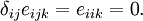
Show the following:

1) $\delta_{ii} = 3$

\delta_{ii} = \delta_{11} + \delta_{22} + \delta_{33} = 1 + 1 + 1 = 3\qquad \implies \qquad \delta_{ii} = 3

2) $e_{ijk}e_{pqk} = \delta_{ip}\delta_{jq} - \delta_{iq}\delta_{jp}$

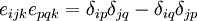
The LHS is

e_{ijk}e_{pqk} = e_{ij1}e_{pq1} + e_{ij2}e_{pq2} + e_{ij3}e_{pq3}

If $i=j$ , then we have

LHS = ({e_{iik}})~~(e_{pqk}) = 0 ~;~~ RHS = \delta_{ip}\delta_{iq} - \delta_{iq}\delta_{ip} = 0

We get the same result if $p=q$ . The only nonzero LHS and RHS occur when $i\ne j$ and $p\ne q$ .

Case 1: $i=1$ , $j=2$ , $p=1$ , $q=2$ .

LHS = ({e_{121}e_{121}})~~ + ({e_{122}e_{122}})~~ + ({e_{123}e_{123}})~~ = 1 ~;~~ RHS = ({\delta_{11}\delta_{11}})~~ - ({\delta_{12}\delta_{12}})~~ = 1

Case 2: $i=1$ , $j=2$ , $p=2$ , $q=1$ or

$i=2$ , $j=1$ , $p=1$ , $q=2$ .

LHS = ({e_{121}e_{211}})~~ + ({e_{122}e_{212}})~~ + ({e_{123}e_{213}})~~ = -1 ~;~~ RHS = ({\delta_{12}\delta_{21}})~~ - ({\delta_{11}\delta_{22}})~~ = -1

Case 3: $i=2$ , $j=1$ , $p=2$ , $q=1$ .

LHS = ({e_{211}e_{211}})~~ + ({e_{212}e_{212}})~~ + ({e_{213}e_{213}})~~ = 1 ~;~~ RHS = ({\delta_{22}\delta_{11}})~~ - ({\delta_{21}\delta_{12}})~~ = 1

Case 4: $i=2$ , $j=3$ , $p=2$ , $q=3$ .

LHS = ({e_{231}e_{231}})~~ + ({e_{232}e_{232}})~~ + ({e_{233}e_{233}})~~ = 1 ~;~~ RHS = ({\delta_{22}\delta_{22}})~~ - ({\delta_{23}\delta_{23}})~~ = 1

Case 5: $i=2$ , $j=3$ , $p=3$ , $q=2$ or

$i=3$ , $j=2$ , $p=2$ , $q=3$ .

LHS = ({e_{231}e_{321}})~~ + ({e_{232}e_{322}})~~ + ({e_{233}e_{323}})~~ = -1 ~;~~ RHS = ({\delta_{23}\delta_{32}})~~ - ({\delta_{22}\delta_{33}})~~ = -1

Case 6: $i=3$ , $j=2$ , $p=3$ , $q=2$ .

LHS = ({e_{321}e_{321}})~~ + ({e_{322}e_{322}})~~ + ({e_{323}e_{323}})~~ = 1 ~;~~ RHS = ({\delta_{33}\delta_{22}})~~ - ({\delta_{32}\delta_{23}})~~ = 1

Case 7: $i=3$ , $j=1$ , $p=3$ , $q=1$ .

LHS = ({e_{311}e_{311}})~~ + ({e_{312}e_{312}})~~ + ({e_{313}e_{313}})~~ = 1 ~;~~ RHS = ({\delta_{33}\delta_{11}})~~ - ({\delta_{31}\delta_{13}})~~ = 1

Case 8: $i=3$ , $j=1$ , $p=1$ , $q=3$ or

$i=1$ , $j=3$ , $p=3$ , $q=1$ .

LHS = ({e_{311}e_{131}})~~ + ({e_{312}e_{132}})~~ + ({e_{313}e_{133}})~~ = -1 ~;~~ RHS = ({\delta_{31}\delta_{13}})~~ - ({\delta_{33}\delta_{11}})~~ = -1

Case 9: $i=1$ , $j=3$ , $p=1$ , $q=3$ .

LHS = ({e_{131}e_{131}})~~ + ({e_{132}e_{132}})~~ + ({e_{133}e_{133}})~~ = 1 ~;~~ RHS = ({\delta_{11}\delta_{33}})~~ - ({\delta_{13}\delta_{31}})~~ = 1

Hence the $~e-\delta$ relation is satisfied for all cases.

3) $\delta_{ij}e_{ijk} = 0$

{ {\delta_{ij}e_{ijk} = e_{iik} = 0 }. }

4) $e_{qrs} d_q d_s = 0$

\begin{align} e_{qrs} d_q d_s = & \sum_{q=1}^3 \sum_{s=1}^3 e_{qrs} d_q d_s \\ = & ({e_{1r1} d_1 d_1})~~~ + e_{1r2} d_1 d_2 + e_{1r3} d_1 d_3 + \\ & e_{2r1} d_2 d_1 + ({e_{2r2} d_2 d_2})~~~ + e_{2r3} d_2 d_3 + \\ & e_{3r1} d_3 d_1 + e_{3r2} d_3 d_2 + ({e_{3r3} d_3 d_3}) \end{align}

For $r=1$ ,

e_{qrs} d_q d_s = ({e_{112}})~~~ d_1 d_2 + ({e_{113}})~~~ d_1 d_3 + ({e_{211}})~~~ d_2 d_1 + ({e_{213}})~~~ d_2 d_3 + ({e_{311}})~~~ d_3 d_1 + ({e_{312}})~~~ d_3 d_2 = 0

For $r=2$ ,

e_{qrs} d_q d_s = ({e_{122}})~~~ d_1 d_2 + ({e_{123}})~~~ d_1 d_3 + ({e_{221}})~~~ d_2 d_1 + ({e_{223}})~~~ d_2 d_3 + ({e_{321}})~~~ d_3 d_1 + ({e_{322}})~~~ d_3 d_2 = 0

For $r=3$ ,

e_{qrs} d_q d_s = ({e_{132}})~~~ d_1 d_2 + ({e_{133}})~~~ d_1 d_3 + ({e_{231}})~~~ d_2 d_1 + ({e_{233}})~~~ d_2 d_3 + ({e_{331}})~~~ d_3 d_1 + ({e_{332}})~~~ d_3 d_2 = 0

Hence shown.

Part 3

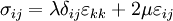
The elasticity tensor is given by

\boldsymbol{\mathsf{C}} = \lambda~ \boldsymbol{\mathit{1}}\otimes\boldsymbol{\mathit{1}} + 2\mu~\boldsymbol{\mathsf{I}}

where $\lambda, \mu$ are Lame constants, $\boldsymbol{\mathit{1}}$ is the second order identity tensor, and $\boldsymbol{\mathsf{I}}$ is the fourth-order symmetric identity tensor. The two identity tensors are defined as

\begin{align} \boldsymbol{\mathit{1}} & = \delta_{ij}~\mathbf{e}_i\otimes\mathbf{e}_j \\ \boldsymbol{\mathsf{I}} & = \frac{1}{2}[\delta_{ik}\delta_{jl} + \delta_{il}\delta_{jk}]~ \mathbf{e}_i\otimes\mathbf{e}_j\otimes\mathbf{e}_k\otimes\mathbf{e}_l \end{align}

The stress-strain relation is

\boldsymbol{\sigma} = \boldsymbol{\mathsf{C}} : \boldsymbol{\varepsilon}

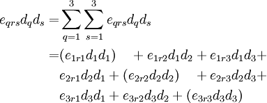
Show that the stress-strain relation can be written in index notation as

\sigma_{ij} = 2\mu\varepsilon_{ij} + \lambda\varepsilon_{kk}\delta_{ij}~.

Write the stress-strain relations in expanded form.

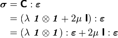
\begin{align} \boldsymbol{\sigma} & = \boldsymbol{\mathsf{C}} : \boldsymbol{\varepsilon} \\ & = \left(\lambda~ \boldsymbol{\mathit{1}}\otimes\boldsymbol{\mathit{1}} + 2\mu~\boldsymbol{\mathsf{I}}\right):\boldsymbol{\varepsilon} \\ & = \left(\lambda~ \boldsymbol{\mathit{1}}\otimes\boldsymbol{\mathit{1}}\right):\boldsymbol{\varepsilon} + 2\mu~\boldsymbol{\mathsf{I}}:\boldsymbol{\varepsilon} \end{align}

Now, in dyadic notation

\boldsymbol{\mathit{1}}\otimes\boldsymbol{\mathit{1}} = (\delta_{ij}~\mathbf{e}_i\otimes\mathbf{e}_j)\otimes (\delta_{kl}~\mathbf{e}_k\otimes\mathbf{e}_l) = \delta_{ij}\delta_{kl}~ \mathbf{e}_i\otimes\mathbf{e}_j\otimes\mathbf{e}_k\otimes\mathbf{e}_l ~\text{and}~ \boldsymbol{\varepsilon} = \varepsilon_{kl}~\mathbf{e}_k\otimes\mathbf{e}_l

Therefore

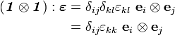
\begin{align} (\boldsymbol{\mathit{1}}\otimes\boldsymbol{\mathit{1}}):\boldsymbol{\varepsilon} & = \delta_{ij}\delta_{kl}\varepsilon_{kl}~\mathbf{e}_i\otimes\mathbf{e}_j \\ & = \delta_{ij}\varepsilon_{kk}~\mathbf{e}_i\otimes\mathbf{e}_j \end{align}

Similarly,

\begin{align} \boldsymbol{\mathsf{I}}:\boldsymbol{\varepsilon} & = \left( \frac{1}{2}[\delta_{ik}\delta_{jl} + \delta_{il}\delta_{jk}] \varepsilon_{kl}\right)~ \mathbf{e}_i\otimes\mathbf{e}_j \\ & = \frac{1}{2}\left(\delta_{ik}\varepsilon_{kj} + \delta_{il}\varepsilon_{jl}\right)~ \mathbf{e}_i\otimes\mathbf{e}_j \\ & = \frac{1}{2}\left(\varepsilon_{ij} + \varepsilon_{ji}\right)~\mathbf{e}_i\otimes\mathbf{e}_j \\ & = \varepsilon_{ij}~ \mathbf{e}_i\otimes\mathbf{e}_j \qquad \text{(symmetry)} \end{align}

The stress-strain law becomes

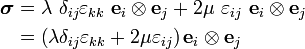
\begin{align} \boldsymbol{\sigma} & = \lambda~\delta_{ij}\varepsilon_{kk}~\mathbf{e}_i\otimes\mathbf{e}_j + 2\mu~ \varepsilon_{ij}~ \mathbf{e}_i\otimes\mathbf{e}_j \\ & = \left(\lambda\delta_{ij}\varepsilon_{kk} + 2\mu\varepsilon_{ij}\right) \mathbf{e}_i\otimes\mathbf{e}_j \end{align}

Expanding the left hand side, we get

\sigma_{ij}~\mathbf{e}_i\otimes\mathbf{e}_j = \left(\lambda\delta_{ij}\varepsilon_{kk} + 2\mu\varepsilon_{ij}\right) \mathbf{e}_i\otimes\mathbf{e}_j

Therefore,

\sigma_{ij} = \lambda\delta_{ij}\varepsilon_{kk} + 2\mu\varepsilon_{ij}

Problem 2: Rotating Vectors and Tensors

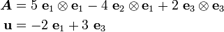
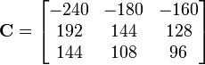
Let ( $\mathbf{e}_1,\mathbf{e}_2,\mathbf{e}_3$ ) be an orthonormal basis. Let $\boldsymbol{A}$ be a second order tensor and $\mathbf{u}$ be a vector with components

\begin{align} \boldsymbol{A} &= 5~\mathbf{e}_1\otimes\mathbf{e}_1 - 4~\mathbf{e}_2\otimes\mathbf{e}_1 + 2~\mathbf{e}_3\otimes\mathbf{e}_3\\ \mathbf{u} &= -2~\mathbf{e}_1 + 3~\mathbf{e}_3 \end{align}

Solution

Part 1

Write out $\boldsymbol{A}$ and $\mathbf{u}$ in matrix notation.

{{ \mathbf{A} = \begin{bmatrix} 5 & 0 & 0 \\ -4 & 0 & 0 \\ 0 & 0 & 2 \end{bmatrix} ; \qquad \mathbf{u} = \begin{bmatrix} -2 \\ 0 \\ 3 \end{bmatrix} }}

Part 2

Find the components of the vector $\mathbf{v} = \boldsymbol{A}\bullet\mathbf{u}$ in the basis ( $\mathbf{e}_1,\mathbf{e}_2,\mathbf{e}_3$ ).

The components of $\mathbf{v}$ are

v_i = A_{ij} u_j

Therefore

v_1 = (5)(-2) = -10 ;~~ v_2 = (-4)(-2) = 8 ;~~ v_3 = (2)(3) = 6

{{ \mathbf{v} = -10~\mathbf{e}_1 + 8 \mathbf{e}_2 + 6 \mathbf{e}_3 }}

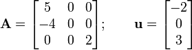
Part 3

Find the components of the vector $\mathbf{w} = \mathbf{v}\times\mathbf{u}$ in the basis ( $\mathbf{e}_1,\mathbf{e}_2,\mathbf{e}_3$ ).

The cross product is given by

\mathbf{w} = \mathbf{v}\times\mathbf{u} = \begin{vmatrix} \mathbf{e}_1 & \mathbf{e}_2 & \mathbf{e}_3 \\ v_1 & v_2 & v_3 \\ u_1 & u_2 & u_3 \end{vmatrix} = \begin{vmatrix} \mathbf{e}_1 & \mathbf{e}_2 & \mathbf{e}_3 \\ -10 & 8 & 6 \\ -2 & 0 & 3 \end{vmatrix} = (8)(3)\mathbf{e}_1 - [(-10)(3)-(6)(-2)]\mathbf{e}_2 - (8)(-2)\mathbf{e}_3

Therefore,

{{ \mathbf{w} = 24~\mathbf{e}_1 + 18 \mathbf{e}_2 + 16 \mathbf{e}_3 }}

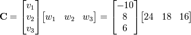
Part 4

Find the components of the tensor $\boldsymbol{C} = \mathbf{v}\otimes\mathbf{w}$ in the orthonormal basis.

The tensor product is given by

\mathbf{v}\otimes\mathbf{w} = v_i w_j ~\mathbf{e}_i\otimes\mathbf{e}_j

Hence, in matrix notation

\mathbf{C} = \begin{bmatrix} v_1 \\ v_2 \\ v_3 \end{bmatrix} \begin{bmatrix} w_1 & w_2 & w_3 \end{bmatrix} = \begin{bmatrix} -10 \\ 8 \\ 6 \end{bmatrix} \begin{bmatrix} 24 & 18 & 16 \end{bmatrix}

{{ \mathbf{C} = \begin{bmatrix} -240 & -180 & -160 \\ 192 & 144 & 128 \\ 144 & 108 & 96 \end{bmatrix} }}

Part 5

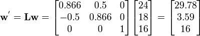
Rotate the basis clockwise by 30 degrees around the $\mathbf{e}_3$ direction. Find the components of $\mathbf{u}$ , $\mathbf{v}$ , $\mathbf{w}$ , and $\boldsymbol{C}$ in the rotated basis.

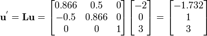
The vector transformation rule is

v^{'}_i = l_{ij} v_i

where $l_{ij}$ are the direction cosines.

In this case, the direction cosines are

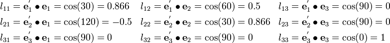
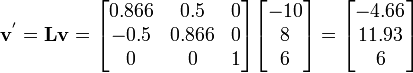
\begin{align} l_{11} & = \mathbf{e}_1^{'}\bullet\mathbf{e}_1 = \cos(30) = 0.866 & l_{12} & = \mathbf{e}_1^{'}\bullet\mathbf{e}_2 = \cos(60) = 0.5& l_{13} & = \mathbf{e}_1^{'}\bullet\mathbf{e}_3 = \cos(90) = 0 \\ l_{21} & = \mathbf{e}_2^{'}\bullet\mathbf{e}_1 = \cos(120) = -0.5 & l_{22} & = \mathbf{e}_2^{'}\bullet\mathbf{e}_2 = \cos(30) = 0.866 & l_{23} & = \mathbf{e}_2^{'}\bullet\mathbf{e}_3 = \cos(90) = 0\\ l_{31} & = \mathbf{e}_3^{'}\bullet\mathbf{e}_1 = \cos(90) = 0& l_{32} & = \mathbf{e}_3^{'}\bullet\mathbf{e}_2 = \cos(90)= 0 & l_{33} & = \mathbf{e}_3^{'}\bullet\mathbf{e}_3 = \cos(0)= 1 \end{align}

Therefore,

\mathbf{u}^{'} = \mathbf{L} \mathbf{u} = \begin{bmatrix} 0.866 & 0.5 & 0 \\ -0.5 & 0.866 & 0 \\ 0 & 0 & 1 \end{bmatrix} \begin{bmatrix} -2 \\ 0 \\ 3 \end{bmatrix} = \begin{bmatrix} -1.732 \\ 1 \\ 3 \end{bmatrix}

{{ \mathbf{u}^{'} = -1.732 \mathbf{e}_1 + 1 \mathbf{e}_2 + 3 \mathbf{e}_3 }}

Similarly,

\mathbf{v}^{'} = \mathbf{L} \mathbf{v} = \begin{bmatrix} 0.866 & 0.5 & 0 \\ -0.5 & 0.866 & 0 \\ 0 & 0 & 1 \end{bmatrix} \begin{bmatrix} -10 \\ 8 \\ 6 \end{bmatrix} = \begin{bmatrix} -4.66 \\ 11.93 \\ 6 \end{bmatrix}

{{ \mathbf{v}^{'} = -4.66 \mathbf{e}_1 + 11.93 \mathbf{e}_2 + 6 \mathbf{e}_3 }}

Also,

\mathbf{w}^{'} = \mathbf{L} \mathbf{w} = \begin{bmatrix} 0.866 & 0.5 & 0 \\ -0.5 & 0.866 & 0 \\ 0 & 0 & 1 \end{bmatrix} \begin{bmatrix} 24 \\ 18 \\ 16 \end{bmatrix} = \begin{bmatrix} 29.78 \\ 3.59 \\ 16 \end{bmatrix}

{{ \mathbf{v}^{'} = 29.78 \mathbf{e}_1 + 3.59 \mathbf{e}_2 + 16 \mathbf{e}_3 }}

From the handout from Slaughter's book, the tensor transformation rule is

T^{'}_{ij} = l_{ip} l_{jq} T_{pq}

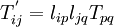
where $l_{ij}$ are the direction cosines.

In matrix form,

\mathbf{T}^{'} = \mathbf{L} \mathbf{T} \mathbf{L}^{T}

Therefore the components of $\boldsymbol{C}$ in the rotated basis are give by

\mathbf{C}^{'} = \begin{bmatrix} 0.866 & 0.5 & 0 \\ -0.5 & 0.866 & 0 \\ 0 & 0 & 1 \end{bmatrix} \begin{bmatrix} -240 & -180 & -160 \\ 192 & 144 & 128 \\ 144 & 108 & 96 \end{bmatrix} \begin{bmatrix} 0.866 & -0.5 & 0 \\ 0.5 & 0.866 & 0 \\ 0 & 0 & 1 \end{bmatrix} = \begin{bmatrix} -138.8 & -16.7 & -74.6 \\ 355.3 &42.8 & 190.9 \\ 178.7 &21.5 & 96 \end{bmatrix}

{{ \mathbf{C}^{'} = \begin{bmatrix} -138.8 & -16.7 & -74.6 \\ 355.3 &42.8 & 190.9 \\ 178.7 &21.5 & 96 \end{bmatrix} }}

Problem 3: More Beams

Part A

Consider a beam of length $L$ = 100 in., cross-section 1 in. $\times$ 1 in., and subjected to a uniformly distributed transverse load $q_0$ lbf/in. Model one half of the beam using symmetry considerations.

Part 1

Hinged-Hinged Beam

The boundary conditions are

w_0(0) = u_0(L/2) = \varphi_x(L/2) = 0 ~.

Compute a plot similar to that shown in Figure 4.3.4 for this case using Beam188 elements. What do you observe?

The result is shown in Table 1.

Table 1. Deflections of a hinged-hinged beam
Load	$U_y$ at $x=L/2$
1	-0.520746
2	-1.04086
3	-1.55922
4	-2.07510
5	-2.58768
6	-3.09622
7	-3.60000
8	-4.09835
9	-4.59065
10	-5.07636

Part 2

Clamped-Clamped Beam

The boundary conditions are

u_0(0) = w_0(0) = \varphi_x(0) = u_0(L/2) = \varphi_{x = L/2} = 0.

Compute a plot for this case using Beam188 elements. Comment on your plot.

The result is shown in Table 2.

Table 2. Deflections of a clamped-clamped beam
Load	$U_y$ at $x=L/2$
1	-0.103456
2	-0.202476
3	-0.294220
4	-0.377753
5	-0.453387
6	-0.521968
7	-0.584455
8	-0.644185
9	-0.696440
10	-0.745243

Listed below is the ANSYS input code for Problem 3A.1 and 3A.2.

/prep7

b = 1
h = 1

et,1,188
sectype,1,beam,rect
secdata,b,h

MP,EX,1,30e6
MP,PRXY,1,0.3

K,1,0,0,0
K,2,50,0,0
k,3,0,50,0

L,1,2,50

latt,1,,1,,3,3,1

LMESH,ALL

!change this section to d,1,all,0 for Problem 3A.2
d,1,uy,0
d,1,uz,0
d,2,rotz,0
nsel,all

sfbeam,all,,pres,10

fini

/solu
nlgeom,on
autots,on
nsubst,10,100,10
outres,all,all
solve
finish

Part B

Part 1

Simulate the unrolling of a cantilever beam from Section 4.1.1 of Ibrahimbegovic (1995) and compare your results with the results shown in the paper.

The result is shown in Table 3.

Table 3. Cantilever free-end displacement components
Load	$U_x$	$U_y$	Rotation
$M=10\pi$	-0.040666	6.3205	-3.1287
$M=20\pi$	9.9578	0.12729	-6.2577

The deformation plots are shown in Figure 4 and 5.

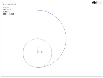Figure 4. Deformed shape under

M=10\pi

for Problem 3B.1.

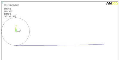Figure 5. Deformed shape under

M=20\pi

for Problem 3B.1.

The ANSYS input code for this problem is listed below.

/prep7

et,1,beam188
sectype,1,beam,rect
secdata,1,1

mp,ex,1,1200
mp,prxy,1,0

l = 10
pi = 4*atan(1)
r = L/2/pi

K,1,0,-r
K,2,-r,0
K,3,0,r
K,4,r,0
K,5,0,-r

k,6,0,0,10

k,7,0,0,0

larc,1,2,7,r,5
larc,2,3,7,r,5
larc,3,4,7,r,5
larc,4,5,7,r,5

latt,1,,1,,6,6,1
lmesh,all

dk,5,all,0

fk,1,mz,-20*pi

/solu
nlgeom,on
cnvtol,f,5,0.001
outres,all,all
arclen,on
nsubst,100
solve
fini

Part 2

Simulate the clamped-hinged deep circular arch from Example 7.3 of Simo and Vu Quoc (1986) and compare you results with the results shown in the paper.

The inputs are: $R = 100$ , $\varphi = 145^o$ , $EI = 10^6$ , and $EA = 100 EI$ . We assume a square cross section. Then

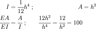
\begin{align} I & = \cfrac{1}{12} h^4~; & A & = h^2 \\ \cfrac{EA}{EI} & = \cfrac{A}{I}~; & \cfrac{12 h^2}{h^4} = \cfrac{12}{h^2} = 100 \end{align}

Therefore, $h = 0.34641$ .

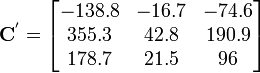
The deformed shape (unconverged) for a load of 905 is shown in Figure 6.

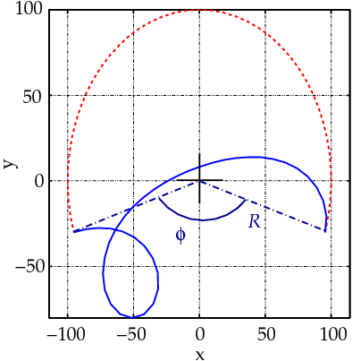Figure 6. Deformed shape of arch.

The load-displacement curve (up to the last converged solution) is shown in Figure 7.

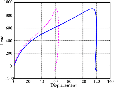Figure 7. Load-displacement plot for circular arch.

The buckling load is 900.925 compared to 905.28 in Simo and Vu Quoc.

The ANSYS file use for the calculations is shown below.

/prep7  
!*
!* Total load
!*
load = 905.0
!*  
!*  Element type
!*
et,1,beam188
keyopt,1,1,0
keyopt,1,2,0
keyopt,1,3,0
keyopt,1,4,0
keyopt,1,6,0
keyopt,1,7,0
keyopt,1,8,0
keyopt,1,9,0
keyopt,1,10,0   
keyopt,1,11,0   
keyopt,1,12,0   
!*
!*  Beam cross-section type
!*
sectype, 1, beam, rect, , 0   
secoffset, cent 
secdata, 0.34641, 0.34641, 0,0,0,0,0,0,0,0 
!*  
!*  Material properties
!* 
mptemp,,,,,,,,  
mptemp,1,0  
mpdata,ex,1,,8.3e8  
mpdata,prxy,1,,0.33 
!*
!* Keypoints
!*
k, 1,   0.000,   0.000, 0.000
k, 2, -95.372, -30.071, 0.000
k ,3,  95.372, -30.071, 0.000 
k ,4,   0.000, 100.000, 0.000
!*  
!* Arcs
!*
larc,3,4,1,100, 
larc,4,2,1,100, 
!*  
!* Element size = 20 elements per arc
!*
lesize,all, , ,20, ,1, , ,1,
!*
!* Mesh the arcs
!*
lmesh, all
!*
!* Plot the nodes
!*
nplot   
/pnum,node,1
/number,0   
/replot 
!*
!* Apply displacement BCs
!*
!* Hinged end
!*
d, 22, ux, 0
d, 22, uy, 0
d, 22, uz, 0
!*
!* Clamped end
!*
d, 1, all, 0
!*
!* Apply load
!*
f, 2, fy, -load
finish  
!*
!* Solve
!*
/solu
antype, static
nlgeom, on
!autots, on
!solcontrol, on
!*
!* Load step 1
!*
time, 1.0
! f, 2, fy, -load
nsubst,100,0,0  
kbc, 0
neqit, 100
outres, ,1
arclen,on,100.0,0.0
lswrite
solve
finish  
!*
!* See solution
!*
/post26
!*
!* Save solution in variables 2 and 3
!*
nsol, 2, 2, u, x               ! Save ux at node 2
nsol, 3, 2, u, y               ! Save uy at node 2
!*
!* Scale solution
!*
prod, 4, 1, , , Load, , ,load  ! Scale time to get load
prod, 5, 2, , ,     , , ,-1    ! Make disp +ve
prod, 6, 3, , ,     , , ,-1    ! Make disp +ve
prvar, 4, 5, 6                 ! Print load, ux, uy
!*
!* Plot solution
!*
/axlab, x, Deflection
/axlab, y, Load
/grid, 1
xvar, 5                     
plvar, 4                       ! plot ux vs load
/noerase
xvar, 6
plvar, 4                       ! plot uy vs load
/erase

Here is another version of solution to this problem.

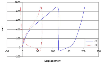Figure 8. Force-displacement diagram for Problem 3B.2.

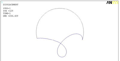Figure 9. Shape deformation at the last load step for Problem 3B.2.

The ANSYS input code for Problem 3B.2 is listed below.

/prep7

A = 1
I = A/100
E = 1e6/I
nu = 0.3

et,1,beam188                ! Element type - BEAM188
sectype,1,beam,asec
secdata,A,I,,I,,2*I

mp,ex,1,E
mp,prxy,1,nu

pi = 4*atan(1)
phi = 35/2/180*pi
x = 100*cos(phi)
y = 100*sin(phi)

k,1,0,0,0
k,2,x,-y,0
k,3,0,100,0
k,4,-x,-y

k,5,0,0,100

larc,2,3,1,100
larc,3,4,1,100
latt,1,,1,,5,5,1

lesize,all,,,40
lmesh,all

dk,2,all,0
dk,4,ux,0
dk,4,uy,0
dk,4,uz,0

fk,3,fy,-900

/solu
nlgeom,on
nsubst,100,0,0
outres,all,all
arclen,on
solve
finish

Part 3

Simulate the buckling of a hinged right-angle frame under both fixed and follower loads from Example 7.4 of Simo and Vu Quoc (1986) and compare your results with those shown in the paper.

The force-displacement diagram is shown in Figure 10. The deformation is illustrated in Figure 11 and 12.

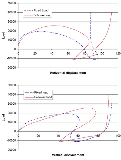Figure 10. Force-displacement diagram for Problem 3B.3.

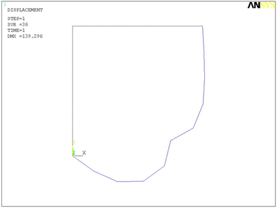Figure 11. Deformation (fixed load) at the last load step for Problem 3B.3.

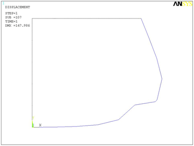Figure 12. Force-displacement diagram (follower load) for Problem 3B.3.

The ANSYS input code for Problem 3B.3 is listed below.

/prep7

et,1,188

E = 7.2e6
I = 2
A = 6

sectype,1,beam,asec
secdata,A,I,,I,,2*I

mp,ex,1,7.2e6
mp,prxy,1,0.3

k,1,0,0,0
k,2,0,120,0
k,3,23,120,0
k,4,26,120,0
k,5,120,120,0

k,6,200,0,0
k,7,0,200,0
l,1,2,5
l,2,3,1
l,3,4,2
l,4,5,4

latt,1,,1,,6,6,1
lmesh,1
latt,1,,1,,7,7,1
lmesh,2,4

d,1,ux,0
d,1,uy,0
d,1,uz,0

d,18,ux,0
d,18,uy,0
d,18,uz,0

esel,s,elem,,7,8

!replace the line below with f,15,fy,-40000 for fixed load

sfbeam,all,,pres,40000/2
esel,all

fini

/solu
nlgeom,on
outres,all,all
arclen,on
nsubst,200
solve
fini

Warning: The arc length method no longer converges with Ansys 13. Try using the stabilization option instead of arclen, on:

stabilize, constant, energy, 0.001, anytime, 0

This article is issued from Wikiversity - version of the Saturday, January 14, 2012. The text is available under the Creative Commons Attribution/Share Alike but additional terms may apply for the media files.