Nonlinear finite elements/Homework 6/Hints
< Nonlinear finite elements < Homework 6Hints for Homework 6: Problem 1: Section 8
Use Maple to reduce your manual labor.
The problem becomes easier to solve if we consider numerical values of the parameters. Let the local nodes numbers of element  be
be  for node , and
  for node
  .
.
Let us assume that the beam is divided into six equal sectors. Then,
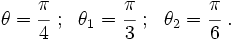
Let  and
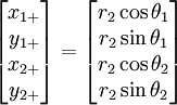
and  . Since the blue point is midway between the two,
  .
.
Also, let the components of the stiffness matrix of the composite be

Let the velocities for nodes and of the element be
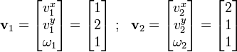
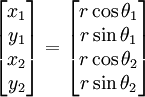
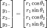
The  and
and  coordinates of the master and slave nodes are
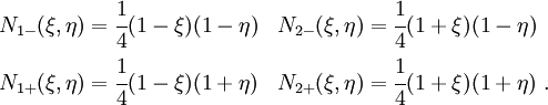
Since there are two master nodes in an element, the parent element is a four-noded quad with shape functions
The isoparametric map is

Therefore, the derivatives with respect to  are
are

Since the blue point is at the center of the element, the values of and  at that point are zero.
Therefore,
at that point are zero.
Therefore,
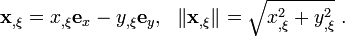
The local laminar basis vector  is given by

The laminar basis vector  is given by

To compute the velocity gradient, we have to find the velocities at the slave nodes using the relation
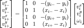
For master node 1 of the element (global node 5), the velocities of the slave nodes are

For master node 2 of the element (global node 6), the velocities of the slave nodes are

The interpolated velocity within the element is given by
![\begin{align}
\mathbf{v}(\boldsymbol{\xi}, t) & = \cfrac{D}{Dt}[\mathbf{x}(\boldsymbol{\xi},t)] \\
& =
\sum_{i- = 1}^2 \frac{\partial }{\partial t}[\mathbf{x}_{i-}(t)]~N_{i^-}(\xi,\eta) +
\sum_{i+ = 1}^2 \frac{\partial }{\partial t}[\mathbf{x}_{i+}(t)]~N_{i^+}(\xi,\eta)\\
& = \sum_{i- = 1}^2 \mathbf{v}_{i-}(t)~N_{i-}(\xi,\eta) +
\sum_{i+ = 1}^2 \mathbf{v}_{i+}(t)~N_{i+}(\xi,\eta) ~.
\end{align}](../I/m/d9011a658fb6e104a874689e6d5d8ea4.png)
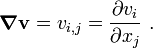
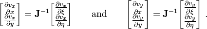
The velocity gradient is given by
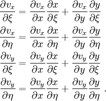
The velocities are given in terms of the parent element coordinates ( ). We have to convert them to the (
 ) system in order to compute the velocity gradient. To do that we recall that
In matrix form
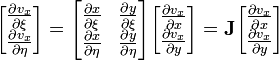
and
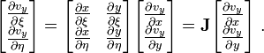
Therefore,
The rate of deformation is given by
![\boldsymbol{D} = \frac{1}{2}[\boldsymbol{\nabla} \mathbf{v} + (\boldsymbol{\nabla} \mathbf{v})^T] ~.](../I/m/e79076c0e4e642bdea962ebf4be11432.png)
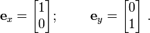
The global base vectors are
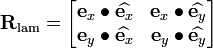
Therefore, the rotation matrix is
Therefore, the components of the rate of deformation tensor with respect to the laminar coordinate system are

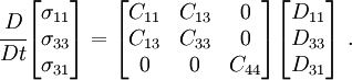
The rate constitutive relation of the material is given by
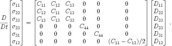
Since the problem is a 2-D one, the reduced constitutive equation is
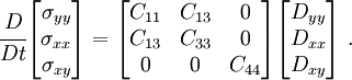
The laminar -direction maps to the composite  -direction and the laminar -directions maps to the composite -direction. Hence the constitutive equation can be written as
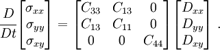
Rearranging,
The plane stress condition requires that  in the laminar coordinate system. We assume that the rate of
  is also zero. In that case, we get
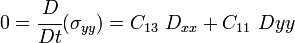
or,
To get the global stress rate and rate of deformation, we have to rotate the components to the global basis using
