Nonlinear finite elements/Homework 2/Solutions

< Nonlinear finite elements < Homework 2

Problem 1: Classification of PDEs

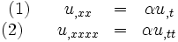
Given:

\begin{matrix} \text{(1)} \qquad u_{,xx}&=&\alpha u_{,t} \\ \text{(2)} \qquad u_{,xxxx}&=&\alpha u_{,tt} \end{matrix}

Solution

Part 1

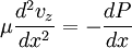
What physical processes do the two PDEs model?

Equation (1) models the one dimensional heat problem where $u(x,t)$ represents temperature at $x$ at time $t$ and $\alpha$ represents the thermal diffusivity.

Equation (2) models the transverse vibrations of a beam. The variable $u(x,t)$ represents the displacement of the point on the beam corresponding to position $x$ at time $t$ . $\alpha$ is $-\frac{\rho A}{EI}$ where $E$ is Young's modulus, $I$ is area moment of inertia, $\rho$ is mass density, and $A$ is area of cross section.

Part 2

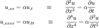
Write out the PDEs in elementary partial differential notation

{ \begin{align} u_{,xx} &= \alpha u_{,t} \qquad \equiv \qquad \frac{\partial ^2u}{\partial x^2}=\alpha \frac{\partial u}{\partial t} \\ u_{,xxxx} &= \alpha u_{,tt}\qquad \equiv \qquad \frac{\partial ^4u}{\partial x^4}=\alpha \frac{\partial ^2u}{\partial t^2} \end{align} }

Part 3

Determine whether the PDEs are elliptic, hyperbolic, or parabolic. Show how you arrived at your classification.

Equation (1) is parabolic for all values of $\alpha$ .

We can see why by writing it out in the form given in the notes on Partial differential equations.

(1) \frac{\partial^2 u}{\partial x^2} + (0) \frac{\partial^2 u}{\partial x\partial t} + (0)\frac{\partial^2 u}{\partial t^2}+ (0) \frac{\partial u}{\partial x} + (-\alpha)\frac{\partial u}{\partial t} +(0) u = 0

Hence, we have $a = 1$ , $b = 0$ , $c = 0$ , $d = 0$ , $e = -\alpha$ , $f = 0$ , and $g = 0$ . Therefore,

{ b^2-4ac = 0-(1)(0)=0 \Rightarrow \text{parabolic} }

Equation (2) is hyperbolic for positive values of $\alpha$ , parabolic when $\alpha$ is zero, and elliptic when $\alpha$ is less than zero.

Problem 2: Models of Physical Problems

Given:

\frac{d}{dx}\left(a(x)\frac{du(x)}{dx}\right)+c(x)u(x)=f(x)\quad \mbox{for }\quad x\in (O,L)

Solution

Heat transfer: : $kA\frac{d^2T}{dx^2}+ap\beta T=f$
Flow through porous medium: : $\mu\frac{d^2\phi}{dx^2}=f$
Flow through pipe: : $\frac{1}{R}\frac{d^2P}{dx^2}=0$
Flow of viscous fluids: : $\mu\frac{d^2v_z}{dx^2}=-\frac{dP}{dx}$
Elastic cables: : $T\frac{d^2u}{dx^2}=f$
Elastic bars: : $EA\frac{d^2u}{dx^2}=f$
Torsion of bars: : $GJ\frac{d^2\theta}{dx^2}=0$
Electrostatics: : $\varepsilon\frac{d^2\phi}{dx^2}=\rho$

Problem 4: Least Squares Method

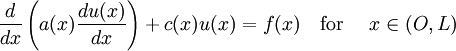
Given:

The residual over an element is

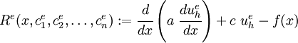
R^e(x,c^e_1,c^e_2,\dots,c^e_n) := \cfrac{d}{dx}\left(a~\cfrac{du^e_h}{dx}\right) + c~u^e_h - f(x)

where

u^e_h(x) = \sum_{j=1}^n c^e_j \varphi^e_j(x) ~.

In the least squares approach, the residual is minimized in the following sense

\frac{\partial }{\partial c_i}\int_{x_a}^{x_b} [R^e(x,c^e_1,c^e_2,\dots,c^e_n)]^2~dx = 0, \qquad i=1,2,\dots,n ~.

Solution

Part 1

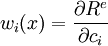
What is the weighting function used in the least squares approach?

We have,

\frac{\partial }{\partial c_i}\int_{x_a}^{x_b} [R^e]^2~dx = \int_{x_a}^{x_b} 2R^e\frac{\partial R^e}{\partial c_i}~dx = 0 ~.

Hence the weighting functions are of the form

{ w_i(x)=\frac{\partial R^e}{\partial c_i} }

Part 2

Develop a least-squares finite element model for the problem.

To make the typing of the following easier, I have gotten rid of the subscript $h$ and the superscript $e$ . Please note that these are implicit in what follows.

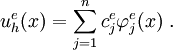
We start with the approximate solution

u(x) = \sum_{j=1}^n c_j \varphi_j(x) ~.

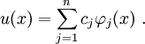
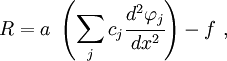
The residual is

R = \cfrac{d}{dx}\left[a~\left(\sum_j c_j\cfrac{d\varphi_j}{dx}\right) \right] + c~\left(\sum_j c_j\varphi_j\right) - f(x) ~.

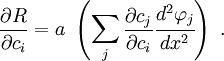
The derivative of the residual is

\frac{\partial R}{\partial c_i} = \cfrac{d}{dx}\left[a~\left(\sum_j \frac{\partial c_j}{\partial c_i} \cfrac{d\varphi_j}{dx}\right) \right] + c~\left(\sum_j \frac{\partial c_j}{\partial c_i}\varphi_j\right) - f(x) ~.

For simplicity, let us assume that $a$ is constant, and $c = 0$ . Then, we have

R = a~\left(\sum_j c_j\cfrac{d^2\varphi_j}{dx^2}\right) - f~,

and

\frac{\partial R}{\partial c_i} = a~\left(\sum_j \frac{\partial c_j}{\partial c_i} \cfrac{d^2\varphi_j}{dx^2}\right) ~.

Now, the coefficients $c_i$ are independent. Hence, their derivatives are

\frac{\partial c_j}{\partial c_i} = \begin{cases} 0 & \text{for} ~~ i \ne j \\ 1 & \text{for} ~~ i = j \end{cases}

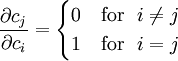
Hence, the weighting functions are

\frac{\partial R}{\partial c_i} = a~\cfrac{d^2\varphi_i}{dx^2} ~.

The product of these two quantities is

R\frac{\partial R}{\partial c_i} = \left(a\sum_j c_j\cfrac{d^2\varphi_j}{dx^2} - f\right) \left(a\cfrac{d^2\varphi_i}{dx^2}\right) = \sum_j \left[ \left(a^2\cfrac{d^2\varphi_i}{dx^2}\cfrac{d^2\varphi_j}{dx^2}\right) c_j \right] - af\cfrac{d^2\varphi_i}{dx^2}~.

Therefore,

\int_{x_a}^{x_b} R\frac{\partial R}{\partial c_i}~dx = 0 \implies \sum_j \left[ \left(\int_{x_a}^{x_b} a^2\cfrac{d^2\varphi_i}{dx^2}\cfrac{d^2\varphi_j}{dx^2}~dx\right) c_j \right] - \int_{x_a}^{x_b} af\cfrac{d^2\varphi_i}{dx^2}~dx = 0

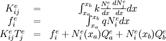
These equations can be written as

K_{ij} c_j = f_i

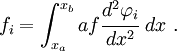
where

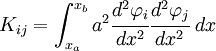
{ K_{ij} = \int_{x_a}^{x_b} a^2\cfrac{d^2\varphi_i}{dx^2}\cfrac{d^2\varphi_j}{dx^2}~dx }

and

{ f_i = \int_{x_a}^{x_b} af\cfrac{d^2\varphi_i}{dx^2}~dx~. }

Part 3

Discuss some functions $(\varphi_j^e)$ that can be used to approximate $u$

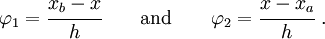
For the least squares method to be a true "finite element" type of method we have to use finite element shape functions. For instance, if each element has two nodes we could choose

\varphi_1 = \cfrac{x_b - x}{h} \qquad \text{and} \qquad \varphi_2 = \cfrac{x - x_a}{h}~.

Another possiblity is set set of polynomials such as

\varphi = \{1, x, x^2, x^3\}~.

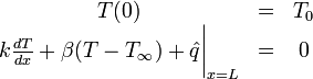
Problem 5: Heat Transefer

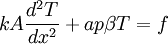
Given:

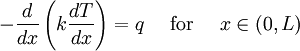
-\frac{d}{dx}\left(k\frac{dT}{dx}\right)=q\quad\mbox{ for }\quad x \in (0,L)

where $T$ is the temperature, $k$ is the thermal conductivity, and $q$ is the heat generation. The Boundary conditions are

\begin{matrix} T(0)&=&T_0\\ k\frac{dT}{dx}+\beta(T-T_\infty)+\hat{q}\bigg |_{x=L}&=&0 \end{matrix}

Solution

Part 1

Formulate the finite element model for this problem over one element

First step is to write the weighted-residual statement

0=\int_{x_a}^{x_b} w_i^e\left[-\frac{d}{dx}\left( k\frac{dT_h^e}{dx}\right)-q\right]dx

Second step is to trade differentiation from $T_h^e$ to $w_i^e$ , using integration by parts. We obtain

0=\int_{x_a}^{x_b} \left(k\frac{w_i^e}{dx}\frac{dT_h^e}{dx}- w_i^eq\right)dx-\left[w_i^ek\frac{dT_h^e}{dx}\right]_{x_a}^{x_b} \text{(3)} \qquad

Rewriting (3) in using the primary variable $T$ and secondary variable $k\frac{dT}{dx}\equiv Q$ as described in the text book to obtain the weak form

0=\int_{x_a}^{x_b} \left(k\frac{w_i^e}{dx}\frac{dT_h^e}{dx}- w_i^eq\right)dx-w_i^e(x_a)Q_a^e-w_i^e(x_b)Q_b^e \text{(4)} \qquad

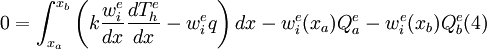
From (4) we have the following

\begin{matrix} K_{ij}^e&=&\int_{x_a}^{x_b} k\frac{N_i^e}{dx}\frac{dN_j^e}{dx}dx\\ f_i^e&=&\int_{x_a}^{x_b} qN_i^edx\\ K_{ij}^eT_j^e&=&f_i^e+N_i^e(x_a)Q_a^e+N_i^e(x_b)Q_b^e \end{matrix}

Part 2

Use ANSYS to solve the problem of heat conduction in an insulated rod. Compare the solution with the exact solution. Try at least three refinements of the mesh to confirm that your solution converges.

The following inputs are used to solve for the solution of this problem:

  /prep7
  pi = 4*atan(1) !compute value for pi
  ET,1,LINK34!convection element
  ET,2,LINK32!conduction element
  R,1,1!AREA = 1
  MP,KXX,1,0.01!conductivity
  MP,HF,1,25 !convectivity
  emax = 2
  length = 0.1
  *do,nnumber,1,emax+1 !begin loop to creat nodes
     n,nnumber,length/emax*(nnumber-1),0
     n,emax+2,length,0!extra node for the convetion element
  *enddo
  type,2 !switch to conduction element
  *do,enumber,1,emax
     e,enumber,enumber+1
  *enddo
  TYPE,1 !switch to convection element
  e,emax+1,emax+2!creat zero length element
  D,1,TEMP,50
  D,emax+2,TEMP,5
  FINISH

  /solu
  solve
  fini

  /post1
  /output,p5,txt
  prnsol,temp
  prnld,heat
  /output,,
  fini

ANSYS gives the following results

Node	Temperature
1	50.000
2	27.590
3	5.1793

Node	Heat Flux
1	-4.4821
4	4.4821

Part 3

Write you own code to solve the problem in part 2.

The following Maple code can be used to solve the problem.

> restart;
> with(linalg):
> L:=0.1:kxx:=0.01:beta:=25:T0:=50:Tinf:=5:
> # Number of elements
> element:=10:
> # Division length
> ndiv:=L/element:
> # Define node location
> for i from 1 to element+1 do
>   x[i]:=ndiv*(i-1);
> od:
> # Define shape function
> for j from 1 to element do
>   N[j][1]:=(x[j+1]-x)/ndiv;
>   N[j][2]:=(x-x[j])/ndiv; 
> od:
> # Create element stiffness matrix
> for k from 1 to element do
>   for i from 1 to 2 do
>     for j from 1 to 2 do
>       Kde[k][i,j]:=int(kxx*diff(N[k][i],x)*diff(N[k][j],x),x=x[k]..x[k+1]); 
>     od;
>   od;
> od;
> Kde[0][2,2]:=0:Kde[element+1][1,1]:=0:
> # Create global matrix for conduction Kdg and convection Khg
> Kdg:=Matrix(1..element+1,1..element+1,shape=symmetric):
> Khg:=Matrix(1..element+1,1..element+1,shape=symmetric):
> for k from 1 to element+1 do
>   Kdg[k,k]:=Kde[k-1][2,2]+Kde[k][1,1];
>   if (k <= element) then
>     Kdg[k,k+1]:=Kde[k][1,2];
>   end if;
> od:
> Khg[element+1,element+1]:=beta:
> # Create global matrix Kg = Kdg + Khg
> Kg:=matadd(Kdg,Khg):
> # Create T and F vectors
> Tvect:=vector(element+1):Fvect:=vector(element+1):
> for i from 1 to element do
>   Tvect[i+1]:=T[i+1]:
>   Fvect[i]:=f[i]:
> od:
> Tvect[1]:=T0:
> Fvect[element+1]:=Tinf*beta:
> # Solve the system Ku=f
> Ku:=multiply(Kg,Tvect):
> # Create new K matrix without first row and column from Kg
> newK:=Matrix(1..element,1..element):
> for i from 1 to element do
>   for j from 1 to element do
>     newK[i,j]:=coeff(Ku[i+1],Tvect[j+1]);
>   od;
> od;
> # Create new f matrix without f1
> newf:=vector(element,0):
> newf[1]:=-Ku[2]+coeff(Ku[2],T[2])*T[2]+coeff(Ku[2],T[3])*T[3]:
> newf[element]:=Tinf*beta:
> # Solve the system newK*T=newf
> solution:=multiply(inverse(newK),newf);
> exact := 50-448.2071713*x;
> with(plots):
> # Warning, the name changecoords has been redefined
> data := [[ x[n+1], solution[n]] <math>n=1..element]:
> FE:=plot(data, x=0..L, style=point,symbol=circle,legend="FE"):
> ELAS:=plot(exact,x=0..L,legend="exact",color=black):
> display({FE,ELAS},title="T(x) vs x",labels=["x","T(x)"]);

This article is issued from Wikiversity - version of the Thursday, March 06, 2008. The text is available under the Creative Commons Attribution/Share Alike but additional terms may apply for the media files.