Nonlinear finite elements/Homework 2

Problem 1: Classification of PDEs

Two commonly encountered PDEs in engineering are

u_{,xx} = \alpha~u_{,t}

and

u_{,xxxx} = \alpha~u_{,tt}

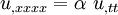
What physical processes do the two PDEs model?
Write out the PDEs in elementary partial differential notation (that is, using symbols of the form $\frac{\partial u}{\partial x}$ ).
Determine whether the PDEs are elliptic, hyperbolic, or parabolic. Show how you arrived at your classification.

Problem 2: Models of Physical Problems

The differential equation which can be written as

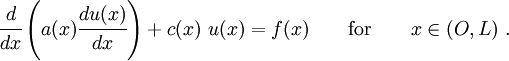
\cfrac{d}{dx}\left(a(x)\cfrac{du(x)}{dx}\right) + c(x)~u(x) = f(x) \qquad \text{for} \qquad x\in(O,L) ~.

arises in a number of fields of physics and engineering.

Write out the ODEs for at least five of these physical situations and identify the meanings of the variables.

Problem 3: Weighted Residual Methods

Give examples from the scientific literature, with full references, where the collocation, subdomain, and least squares weighted residual methods have been used.

Explain why the standard finite element method has not been used in these examples.

One example for each method will suffice.

Problem 4: Least Squares Method

The residual over an element (for the general second-order ODE) is defined as

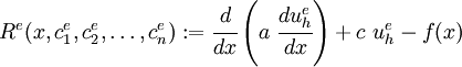
R^e(x,c^e_1,c^e_2,\dots,c^e_n) := \cfrac{d}{dx}\left(a~\cfrac{du^e_h}{dx}\right) + c~u^e_h - f(x)

where

u^e_h(x) = \sum_{j=1}^n c^e_j \varphi^e_j(x) ~.

In the least squares method, the residual $R^e$ is minimized in the following sense:

\frac{\partial }{\partial c_i}\int_{x_a}^{x_b} [R^e(x,c^e_1,c^e_2,\dots,c^e_n)]^2~dx = 0, \qquad i=1,2,\dots,n ~.

What is the weighting function used in the least squares approach?
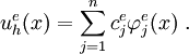
Develop a least-squares finite element model for the problem. You don't have to find the solution to a specific problem - just the components of $\mathbf{K}$ , $\mathbf{u}$ , and $\mathbf{f}$ for an element will do.
Discuss some functions ( $\varphi^e_j$ ) that can be used to approximate $u$ .

Problem 5: Heat Transfer

The differential equation that is used to model one-dimensional heat transfer is

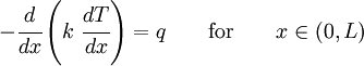
-\cfrac{d}{dx}\left(k~\cfrac{dT}{dx}\right) = q \qquad \text{for} \qquad x \in (0,L)

where $T$ is the temperature, $k$ is the thermal conductivity, and $q$ is the heat generation.

Let us assume that the boundary conditions are

\begin{align} T(0) &= T_0 \\ \left.\left[ k\cfrac{dT}{dx}+\beta~(T - T_{\infty})+\hat{q}\right] \right|_{x=L} & = 0 \end{align}

where $T_0$ is a prescribed temperature, $\beta$ is a convective heat transfer coefficient, $T_{\infty}$ is the ambient temperature, and $\hat{q}$ is a prescribed heat flux.

Formulate the finite element model for this problem over one element, that is, find expressions for the stiffness matrix and the load vector.
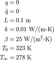
Use ANSYS (or any other software tool) to solve the problem of heat conduction in an insulated rod. Compare your solution with the exact solution (if available). Try at least three refinements of the mesh to confirm that your solution converges.
Write your own code to solve the problem in part 2 (use two elements). Compare your solution with the ANSYS (or other software) solution.

Use the following data:

\begin{align} q & = 0 \\ \hat{q} & = 0 \\ L & = 0.1~\text{m} \\ k & = 0.01~\text{W/(m-K)} \\ \beta & = 25~\text{W/(m}^2\text{-K)} \\ T_0 & = 323 ~\text{K} \\ T_{\infty} & = 278 ~\text{K} \end{align}

You can look at the 1-D heat conduction problem on the Introduction to Ansys page to see how ANSYS deals with heat conduction.

This article is issued from Wikiversity - version of the Tuesday, January 08, 2008. The text is available under the Creative Commons Attribution/Share Alike but additional terms may apply for the media files.