Nonlinear finite elements/Effect of mesh distortion

An Example: Effect of Mesh Distortion

Consider the three-noded quadratic displacement element shown in Figure 1.

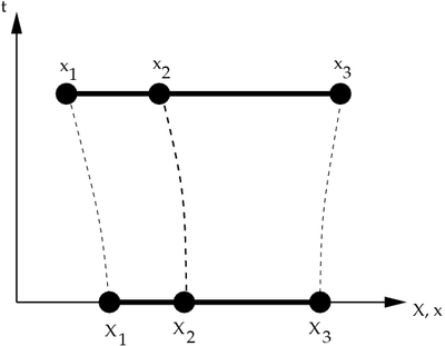Figure 1. Reference and Current Configurations of a 3-noded element.

The shape functions for the parent element are

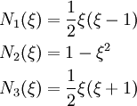
\begin{align} N_1(\xi) & = \frac{1}{2}\xi(\xi-1) \\ N_2(\xi) & = 1-\xi^2 \\ N_3(\xi) & = \frac{1}{2}\xi(\xi+1) \end{align}

In matrix form,

\mathbf{N}(\xi) = \begin{bmatrix} \frac{1}{2}\xi(\xi-1) & 1-\xi^2 & \frac{1}{2}\xi(\xi+1) \end{bmatrix} ~.

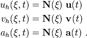
The trial functions (in terms of the parent coordinates) are

\begin{align} u_h(\xi, t) & = \mathbf{N}(\xi)~\mathbf{u}(t) \\ v_h(\xi, t) & = \mathbf{N}(\xi)~\mathbf{v}(t) \\ a_h(\xi, t) & = \mathbf{N}(\xi)~\mathbf{a}(t) ~. \end{align}

The mapping from the Eulerian coordinates to the parent element coordinates is

x(\xi, t) = N_1(\xi)~x_1(t) + N_2(\xi)~x_2(t) + N_3(\xi)~x_3(t) ~.

In matrix form,

x(\xi, t) = \mathbf{N}(\xi)~\mathbf{x}(t)~.

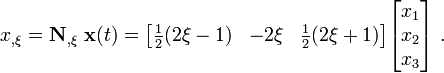
Therefore, the derivative with respect to $\xi$ is

x_{,\xi} = N_{1,\xi}~x_1(t) + N_{2,\xi}~x_2(t) + N_{3,\xi}~x_3(t) = \frac{1}{2}(2\xi-1)~x_1 - 2\xi~x_2 + \frac{1}{2}(2\xi+1)~x_3 ~.

In matrix form,

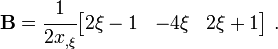
x_{,\xi} = \mathbf{N}_{,\xi}~\mathbf{x}(t) = \begin{bmatrix} \frac{1}{2}(2\xi-1) & - 2\xi & \frac{1}{2}(2\xi+1) \end{bmatrix} \begin{bmatrix} x_1 \\ x_2 \\ x_3 \end{bmatrix}~.

Now, the $\mathbf{B}$ matrix is given by

\mathbf{B} = \mathbf{N}_{,\xi} (x_{,\xi})^{-1} ~.

Therefore,

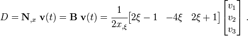
\mathbf{B} = \cfrac{1}{2 x_{,\xi}} \begin{bmatrix} 2\xi-1 & - 4\xi & 2\xi+1 \end{bmatrix} ~.

The rate of deformation is then given by

{ D = \mathbf{N}_{,x}~\mathbf{v}(t) = \mathbf{B}~\mathbf{v}(t) = \cfrac{1}{2 x_{,\xi}} \begin{bmatrix} 2\xi-1 & - 4\xi & 2\xi+1 \end{bmatrix} \begin{bmatrix} v_1 \\ v_2 \\ v_3 \end{bmatrix} ~. }

The stress can be calculated using the relation

\sigma = E^{\sigma D}~D ~.

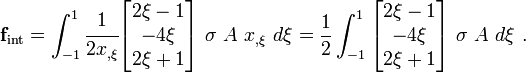
The internal forces are given by

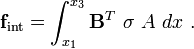
\mathbf{f}_{\text{int}} = \int_{x_1}^{x_3} \mathbf{B}^T~\sigma~A~dx ~.

Plugging in the expression for $\mathbf{B}$ , and changing the limits of integration, we get

{ \mathbf{f}_{\text{int}} = \int_{-1}^{1} \cfrac{1}{2 x_{,\xi}} \begin{bmatrix} 2\xi-1 \\ - 4\xi \\ 2\xi+1 \end{bmatrix} ~\sigma~A~x_{,\xi}~d\xi = \frac{1}{2}\int_{-1}^{1}\begin{bmatrix} 2\xi-1 \\ - 4\xi \\ 2\xi+1 \end{bmatrix}~\sigma~A~d\xi ~. }

If node $2$ is midway between node $1$ and node $3$ ,

x_2 = \frac{1}{2}(x_1 + x_3) ~.

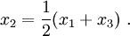
Then we have,

x_{,\xi} = \frac{1}{2}(2\xi-1)~x_1 - \xi~(x_1+x_3) + \frac{1}{2}(2\xi+1)~x_3 = \frac{1}{2}(x_3-x_1) ~.

The rate of deformation becomes

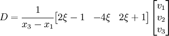
D = \cfrac{1}{x_3-x_1} \begin{bmatrix} 2\xi-1 & - 4\xi & 2\xi+1 \end{bmatrix} \begin{bmatrix} v_1 \\ v_2 \\ v_3 \end{bmatrix}

which is a linear function of $\xi$ .

However, if node $2$ moves away from the middle during deformation, then $x_{,\xi}$ is no longer constant and can become zero or negative. Under such situations the rate of deformation is either infinite or the element inverts upon itself since the isoparametric map is no longer one-to-one.

Let us consider the case where $x_{,\xi}$ is zero. In that case, the Jacobian becomes

J = \cfrac{A}{A_0} x_{,X} = \cfrac{A}{A_0} x_{,\xi}~(X_{,\xi})^{-1} = 0 ~.

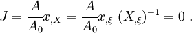
Similarly, when $x_{,\xi}$ is negative, $J$ is negative. This implies that the conservation of mass is violated.

To find the location of $x_2$ when this happens, we set the relation for $x_{,\xi}$ to zero. Then we get,

\frac{1}{2}(2\xi-1)~x_1 - \xi~(x_1+x_3) + \frac{1}{2}(2\xi+1)~x_3 = 0 \qquad \implies \qquad x_2 = \cfrac{x_1+x_3}{2} + \cfrac{x_3-x_1}{4\xi}~.

If $x_{,\xi} = 0$ at $\xi = 1$ , then

x_2 = \cfrac{x_1+3x_3}{4}~.

This means that as node $2$ gets closer and closer to node $3$ , the rate of deformation become infinite at node $3$ and then negative.

If $x_{,\xi} = 0$ at $\xi = -1$ , then

x_2 = \cfrac{3x_1+x_3}{4}~.

This means that as node $2$ gets closer and closer to node $1$ , the rate of deformation becomes infinite at node $1$ and then negative.

These effects of mesh distortion can be severe in multiple dimensions. That is the reason that linear elements are preferred in large deformation simulations.

This article is issued from Wikiversity - version of the Tuesday, November 23, 2010. The text is available under the Creative Commons Attribution/Share Alike but additional terms may apply for the media files.