Nonlinear finite elements/Calculus of variations

< Nonlinear finite elements

Ideas from the calculus of variations are commonly found in papers dealing with the finite element method. This handout discusses some of the basic notations and concepts of variational calculus. Most of the examples are from Variational Methods in Mechanics by T. Mura and T. Koya, Oxford University Press, 1992.

The calculus of variations is a sort of generalization of the calculus that you all know. The goal of variational calculus is to find the curve or surface that minimizes a given function. This function is usually a function of other functions and is also called a functional.

Maxima and minima of functions

The calculus of variations extends the ideas of maxima and minima of functions to functionals.

For a function of one variable $f(x)$ , the minimum occurs at some point $x_{\text{min}}$ . For a functional, instead of a point minimum, we think in terms of a function that minimizes the functional. Thus, for a functional $I[f(x)]$ we can have a minimizing function $f_{\text{min}}(x)$ .

The problem of finding extrema (minima and maxima) or points of inflection (saddle points) can either be constrained or unconstrained.

The unconstrained problem.

Suppose $f(x)$ is a function of one variable. We want to find the maxima, minima, and points of inflection for this function. No additional constraints are imposed on the function. Then, from elementary calculus, the function $f(x)$ has

a minimum if $\cfrac{df}{dx} = 0$ and $\cfrac{d^2 f}{dx^2} > 0$ .
a maximum if $\cfrac{df}{dx} = 0$ and $\cfrac{d^2 f}{dx^2} < 0$ .
a point of inflection if $\cfrac{d^2 f}{dx^2} = 0$ .

Any point where the condition $\cfrac{df}{dx} = 0$ is satisfied is called a stationary point and we say that the function is stationary at that point.

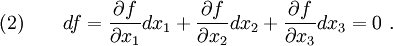
A similar concept is used when the function is of the form $f(x_1,x_2,x_3,t)$ . Then, the function $f$ is stationary if

df = \frac{\partial f}{\partial x_1} dx_1 + \frac{\partial f}{\partial x_2} dx_2 + \frac{\partial f}{\partial x_3} dx_3 + \frac{\partial f}{\partial t} dt = 0~.

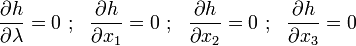
Since $x_1$ , $x_2$ , $x_3$ , and $t$ are independent variables, we can write the stationarity condition as

\frac{\partial f}{\partial x_1} = 0 ~;~~ \frac{\partial f}{\partial x_2} = 0 ~;~~ \frac{\partial f}{\partial x_3} = 0 ~;~~ \frac{\partial f}{\partial t} = 0~.

The constrained problem - Lagrange multipliers.

Suppose we have a function $f(x_1,x_2,x_3)$ . We want to find the minimum (or maximum) of the function $f$ with the added constraint that

\text{(1)} \qquad g(x_1,x_2,x_3) = 0 ~.

The added constraint is equivalent to saying that the variables $x_1$ , $x_2$ , and $x_3$ are not independent and we can write one of the variables in terms of the other two.

The stationarity condition for $f$ is

\text{(2)} \qquad df = \frac{\partial f}{\partial x_1} dx_1 + \frac{\partial f}{\partial x_2} dx_2 + \frac{\partial f}{\partial x_3} dx_3 = 0~.

Since the variables $x_1$ , $x_2$ , and $x_3$ are not independent, the coefficients of $dx_1$ , $dx_2$ , and $dx_3$ are not zero.

At this stage we could express $x_3$ in terms of $x_1$ and $x_2$ using the constraint equation (1), form another stationarity condition involving only $x_1$ and $x_2$ , and set the coefficients of $dx_1$ and $dx_2$ to zero. However, it is usually impossible to solve equation (1) analytically for $x_3$ . Hence, we use a more convenient approach called the Lagrange multiplier method.

Lagrange multiplier method.

From equation (1) we have

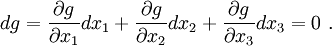
dg = \frac{\partial g}{\partial x_1} dx_1 + \frac{\partial g}{\partial x_2} dx_2 + \frac{\partial g}{\partial x_3} dx_3 = 0~.

We introduce a parameter $\lambda$ called the Lagrange multiplier and using equation (2) we get

df + \lambda dg = 0~.

Then we have,

\left(\frac{\partial f}{\partial x_1} + \lambda\frac{\partial g}{\partial x_1}\right) dx_1 + \left(\frac{\partial f}{\partial x_2} + \lambda\frac{\partial g}{\partial x_2}\right) dx_2 + \left(\frac{\partial f}{\partial x_3} + \lambda\frac{\partial g}{\partial x_3}\right) dx_3 = 0~.

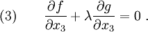
We choose the parameter $\lambda$ such that

\text{(3)} \qquad \frac{\partial f}{\partial x_3} + \lambda\frac{\partial g}{\partial x_3} = 0~.

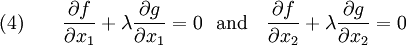
Then, because $x_1$ and $x_2$ are independent, we must have

\text{(4)} \qquad \frac{\partial f}{\partial x_1} + \lambda\frac{\partial g}{\partial x_1} = 0 ~~\text{and}~~~ \frac{\partial f}{\partial x_2} + \lambda\frac{\partial g}{\partial x_2} = 0

We can now use equations (1), (3), and (4) to solve for the extremum point and the Lagrange multiplier. The constraint is satisfied in the process.

Notice that equations (1), (3) and (4) can also be written as

{ \frac{\partial h}{\partial \lambda} = 0 ~;~~ \frac{\partial h}{\partial x_1} = 0 ~;~~ \frac{\partial h}{\partial x_2} = 0 ~;~~ \frac{\partial h}{\partial x_3} = 0 }

where

{ h(x_1, x_2, x_3, \lambda) := f(x_1,x_2,x_3) + \lambda g(x_1,x_2,x_3)~. }

Minima of functionals

Consider the functional

\text{(5)} \qquad I[y(x)] = \int_{x_0}^{x_1} \left[f(x)\left(\cfrac{dy(x)}{dx}\right)^2 + g(x)y(x)^2 + 2h(x)y(x)\right] ~dx~.

We wish to minimize the functional $I$ with the constraints (prescribed boundary conditions)

y(x_0) = y_0 ~,~~~~ y(x_1) = y_1~.

Let the function $y = y(x)$ minimize $I$ . Let us also choose a trial function (that is not quite equal to the solution $y(x)$ )

\text{(6)} \qquad y = y(x) + \lambda v(x)

where $\lambda$ is a parameter, and $v(x)$ is an arbitrary continuous function that has the property that

v(x_0) = 0 ~~\text{and}~~ v(x_1) = 0~.

(See Figure 1 for a geometric interpretation.)

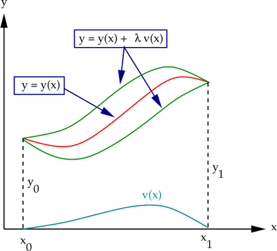Figure 1. Minimizing function

y(x)

and trial functions.

Plug (6) into (5) to get

\text{(8)} \qquad I[y(x)+\lambda v(x)] = \int_{x_0}^{x_1} \left[f(x)\left(\cfrac{dy(x)}{dx}+ \lambda\cfrac{dv}{dx}\right)^2 + g(x)\left[y(x) + \lambda v(x)\right]^2 + 2h(x)\left[y(x) + \lambda v(x)\right]\right] ~dx~.

You can show that equation (8) can be written as (show this)

I[y(x)+\lambda v(x)] = I[y(x)] + \delta I + \delta^2 I ~~~~\text{or,}~~~~ I[y(x)+\lambda v(x)] - I[y(x)] = \delta I + \delta^2 I

where

\text{(9)} \qquad \delta I = 2\lambda \int_{x_0}^{x_1} \left[f(x) \left(\cfrac{dy(x)}{dx}\right) \left(\cfrac{dv(x)}{dx}\right) + g(x) y(x) v(x) + h(x) v(x)\right]~dx

and

\text{(10)} \qquad \delta^2 I = \lambda^2 \int_{x_0}^{x_1} \left[f(x)\left(\cfrac{dv(x)}{dx}\right)^2 + g(x)[v(x)]^2\right]~dx~.

The quantity $\delta I$ is called the first variation of $I$ and the quantity $\delta^2 I$ is called the second variation of $I$ . Notice that $\delta I$ consists only of terms containing $\lambda$ while $\delta^2 I$ consists only of terms containing $\lambda^2$ .

The necessary condition for $I[y(x)]$ to be a minimum is

\text{(11)} \qquad { \delta I = 0 ~. }

Remark.

The first variation of the functional $I[y]$ in the direction $v$ is defined as

{ \delta I(y;v) = \lim_{\epsilon\rightarrow 0} \cfrac{I[y + \epsilon v] - I[y]}{\epsilon} \equiv \left.\cfrac{d}{d\epsilon} I[y + \epsilon v]\right|_{\epsilon = 0} ~.}

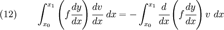
To find which function makes $\delta I$ zero, we first integrate the first term of equation (9) by parts. We have,

\int_{x_0}^{x_1} \left(f \cfrac{dy}{dx}\right) \cfrac{dv}{dx}~dx = \left[\left(f \cfrac{dy}{dx}\right) v \right]_{x_0}^{x_1} - \int_{x_0}^{x_1} \cfrac{d}{dx}\left(f \cfrac{dy}{dx}\right) v~dx~.

Since $v = 0$ at $x_0$ and $x_1$ , we have

\text{(12)} \qquad \int_{x_0}^{x_1} \left(f \cfrac{dy}{dx}\right) \cfrac{dv}{dx}~dx = - \int_{x_0}^{x_1} \cfrac{d}{dx}\left(f \cfrac{dy}{dx}\right) v~dx

Plugging equation (12) into (9) and applying the minimizing condition (11), we get

0 = \int_{x_0}^{x_1} \left[-\cfrac{d}{dx}\left(f(x) \cfrac{dy(x)}{dx}\right) v(x) + g(x) y(x) v(x) + h(x) v(x)\right]~dx

or,

\text{(13)} \qquad \int_{x_0}^{x_1} \left[-\cfrac{d}{dx}\left(f(x) \cfrac{dy(x)}{dx}\right) + g(x) y(x) + h(x) \right]v(x)~dx = 0~.

The fundamental lemma of variational calculus states that if $u(x)$ is a piecewise continuous function of $x$ and $v(x)$ is a continuous function that vanishes on the boundary, then

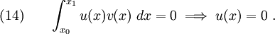
\text{(14)} \qquad { \int_{x_0}^{x_1} u(x) v(x) ~dx = 0 \implies u(x) = 0 ~. }

Applying (14) to (13) we get

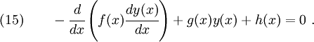
\text{(15)} \qquad -\cfrac{d}{dx}\left(f(x)\cfrac{dy(x)}{dx}\right) + g(x) y(x) + h(x) = 0~.

Equation (15) is called the Euler equation of the functional $I$ . The solution of the Euler equation is the minimizing function that we seek.

Of course, we cannot be sure that the solution represents and minimum unless we check the second variation $\delta^2 I$ . From equation (10) we can see that $\delta^2 I > 0$ if $f(x) > 0$ and $g(x) > 0$ and in that case the problem is guaranteed to be a minimization problem.

We often define

\delta y := \lambda v(x) ~~~\text{and}~~~ \delta y^{'} := \lambda \cfrac{dv(x)}{dx}

where $\delta y$ is called a variation of $y(x)$ .

In this notation, equation (9) can be written as

\delta I = 2\int_{x_0}^{x_1}\left[f\left(\cfrac{dy}{dx}\right)\delta y^{'} + g y \delta y + h \delta y\right]~dx

You see this notation in the principle of virtual work in the mechanics of materials.

An example

Consider the string of length $l$ under a tension $T$ (see Figure 2). When a vertical load $f$ is applied, the string deforms by an amount $u(x)$ in the $y$ -direction. The deformed length of an element $dx$ of the string is

ds = \sqrt{1 + \left(\cfrac{du}{dx}\right)^2} dx ~.

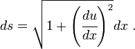
If the deformation is small, we can expand the relation into a Taylor series and ignore the higher order terms to get

ds = \left[1 + \frac{1}{2}\left(\cfrac{du}{dx}\right)^2\right] dx ~.

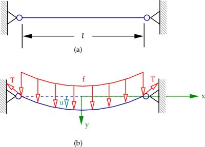Figure 2. An elastic string under a transverse load.

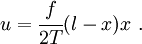
The force T in the string moves a distance

ds - dx = \frac{1}{2}\left(\cfrac{du}{dx}\right)^2~dx.

Therefore, the work done by the force $T$ (per unit original length of the string) (the stored elastic energy) is

\frac{1}{2} T \left(\cfrac{du}{dx}\right)^2~.

The work done by the forces $f$ (per unit original length of string) is

f u

We want to minimize the total energy. Therefore, the functional to be minimized is

I[y] = \cfrac{T}{2} \int_0^l \left(\cfrac{du}{dx}\right)^2~dx - \int_0^l f u~dx ~.

The Euler equation is

T\cfrac{d^2 u}{dx^2} + f = 0~.

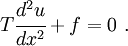
The solution is

u = \cfrac{f}{2T} (l - x) x~.

This article is issued from Wikiversity - version of the Sunday, November 04, 2012. The text is available under the Creative Commons Attribution/Share Alike but additional terms may apply for the media files.