Nonlinear finite elements/Bubnov Galerkin method
< Nonlinear finite elements(Bubnov)-Galerkin Method for Problem 2
The Bubnov-Galerkin method is the most widely used weighted average method. This method is the basis of most finite element methods.
The finite-dimensional Galerkin form of the problem statement of our second order ODE is :
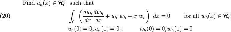
Since the basis functions ( ) are known and linearly independent, the approximate solution
  is completely determined once the constants (
 ) are known.
The Galerkin method provides a great way of constructing solutions. But the question is: how do we choose so that these functions are not only linearly independent but arbitrary? Since the solution is expressed as a sum of these functions, the accuracy of our result depends strongly on the choice of .
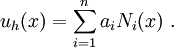
Let the trial solution take the form,
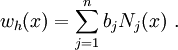
According to the Bubnov-Galerkin approach, the weighting function also takes a similar form
Plug these values into the weak form to get
![\int^1_0 \left[\left(\sum_{i=1}^n a_i\cfrac{dN_i}{dx}\right)
\left(\sum_{j=1}^n b_j\cfrac{dN_j}{dx}\right) +
\left(\sum_{i=1}^n a_i N_i\right)
\left(\sum_{j=1}^n b_j N_j \right) -
x \left(\sum_{j=1}^n b_j N_j\right)\right]~dx = 0](../I/m/d85f0965ef03593abbd8bab6c60ff1e9.png)
or
![\int^1_0 \left[\sum_{j=1}^n b_j
\left(\cfrac{dN_j}{dx} \sum_{i=1}^n a_i\cfrac{dN_i}{dx} +
N_j \sum_{i=1}^n a_i N_i -
x~N_j
\right)
\right] ~dx = 0](../I/m/a2bacabb4daf3111ffb02548c5f21ddb.png)
or
![\int^1_0 \left[\sum_{j=1}^n b_j
\left(\sum_{i=1}^n \left(a_i\cfrac{dN_j}{dx} \cfrac{dN_i}{dx} +
a_i N_j N_i\right) - x~N_j
\right)
\right] ~dx = 0 ~.](../I/m/856cd2d93d5348ab45cceb565f14269d.png)
Taking the sums and constants outside the integrals and rearranging, we get
![\sum_{j=1}^n b_j \left[\sum_{i=1}^n a_i \int^1_0
\left(\cfrac{dN_i}{dx} \cfrac{dN_j}{dx} +
N_i N_j\right)~dx - \int^1_0 x~N_j~dx \right] = 0 ~.](../I/m/56940b74fe499a5722038a2db36003cd.png)
Since the  s are arbitrary, the quantity inside the square brackets must be zero. That is

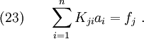
Let us define

Then we get a set of simultaneous linear equations
In matrix form,
