Nonlinear finite elements/Axially loaded bar

An axially loaded bar

Let us consider the simplest solid mechanics problem that we can think of - the axial loading of a bar (see Figure 1).

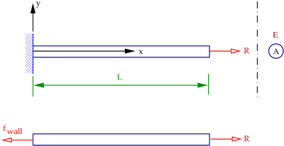Figure 1. Axial loading of a bar.

Given:

The bar is of length $L\,$ and has an area of cross-section $A\,$ . The Young's modulus of the material is $E\,$ .

Find:

We want to find the stresses and deformations in the bar due to the concentrated axial load $\mathbf{R}$ at the end.

Assumptions:

The cross-section of the bar does not change after loading.
The material is linear elastic, isotropic, and homogeneous.
The load is centric.
End-effects are not of interest to us.

Strength of Materials Approach

From the free-body diagram of the bar, a balance of forces gives

\mathbf{f}_{\text{wall}} = \mathbf{R} = \mathbf{f}(\mathbf{x}) ~.

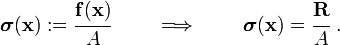
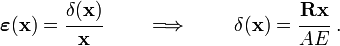
The stress in the bar is given by

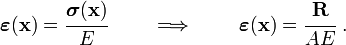
\boldsymbol{\sigma}(\mathbf{x}) := \cfrac{\mathbf{f}(\mathbf{x})}{A} \qquad \implies \qquad {\boldsymbol{\sigma}(\mathbf{x}) = \cfrac{\mathbf{R}}{A}} ~.

The constitutive model for the bar is given by Hooke's law ( $\boldsymbol{\sigma} = E\boldsymbol{\varepsilon}$ ). Therefore, the strain in the bar is

\boldsymbol{\varepsilon}(\mathbf{x}) = \cfrac{\boldsymbol{\sigma}(\mathbf{x})}{E} \qquad \implies \qquad {\boldsymbol{\varepsilon}(\mathbf{x}) = \cfrac{\mathbf{R}}{AE} }~.

To get the deformation of the bar, we use the strain-displacement relations

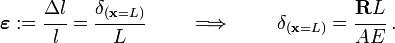
\boldsymbol{\varepsilon} := \cfrac{\Delta l}{l} = \cfrac{\delta_{(\mathbf{x} = L)}}{L} \qquad \implies \qquad {\delta_{(\mathbf{x} = L)} = \cfrac{\mathbf{R} L}{A E} }~.

We can get the deformation of any point in the bar in a similar manner:

\boldsymbol{\varepsilon}(\mathbf{x}) = \cfrac{\delta(\mathbf{x})}{\mathbf{x}} \qquad \implies \qquad {\delta(\mathbf{x}) = \cfrac{\mathbf{R} \mathbf{x}}{A E} }~.

A more complicated axial load

Now, suppose that we have a linear distributed axial load $\mathbf{q}(\mathbf{x}) = a \mathbf{x}$ in addition to the load $\mathbf{R}$ (see Figure 2(a)). This load has units of force per unit length and is also called a body load. Examples are gravity and inertial forces due to rotation around the $y$ axis.

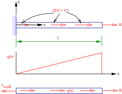Figure 2(a). Distributed axial load

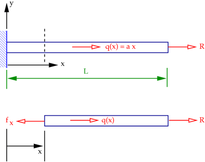Figure 2(b). Free body diagram for distributed axial load

Once again, we want to calculate stresses and displacements. Note that stresses are no longer constant along the length of the bar.

Strength of Materials Approach

From the free body diagram of the bar, a balance of forces gives

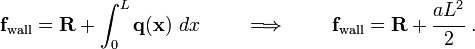
\mathbf{f}_{\text{wall}} = \mathbf{R} + \int_0^L \mathbf{q}(\mathbf{x})~dx \qquad \implies \qquad {\mathbf{f}_{\text{wall}} = \mathbf{R} + \cfrac{a L^2}{2}} ~.

So we know the reaction force at the wall. But we want to know the stress and displacement at any point along the bar.

To do this, we can make a cut at any point along the length and use the free body diagram to compute a reaction force $\mathbf{f}(\mathbf{x})$ (see Figure 2(b)). But this is tedious since we have to repeat the process for every point in the bar.

This article is issued from Wikiversity - version of the Sunday, August 12, 2007. The text is available under the Creative Commons Attribution/Share Alike but additional terms may apply for the media files.