Nonlinear finite elements/Axial bar strong form
< Nonlinear finite elementsAxially loaded bar: Strong Form
In this case, we consider an infinitesimal slice of the bar and perform a balance of forces on that slice (see Figure 1).
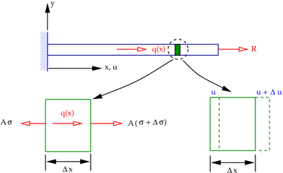 Figure 1. Continuum approach for the axial loading of a bar. |
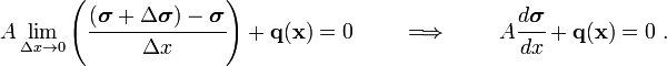
A balance of forces gives

Taking the limit as  , we get
This is a differential equation written in terms of stress. We want to express it in terms of displacements. How do we do this?
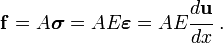
First, we convert the stresses into strains using the constitutive equation
( ).
).
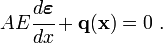
Then, we convert the strains into displacements using the strain-displacement relations:

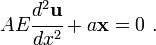
The differential equation in terms of the displacement  is
is
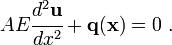
Since  , we have an inhomogeneous ordinary differential equation for the displacements in the bar.
If we can find the displacements in the bar, then we can solve for the strains and therefore the stresses. But to do that, we have to solve the governing differential equation.
To get a unique solution, we need to provide boundary conditions. In this case, these are
- At
 (wall),
  . This is an essential BC.
 - At
 (end),
  . This is a natural BC.
Since the ODE is in terms of , the BCs must also be in terms of . But we have a force at one end. This force has to be converted into an equivalent displacement. How?
Therefore, the BCs become
- At (wall), .
- At (end),
 .
.
The problem can then be stated as
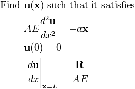
The differential formulation is also called the strong form of the problem.
Analytical Solution
The analytical solution strategy is as follows:
- Set right hand side to zero and solve ( Homogeneous solution).
- Find one solution with RHS =
 ( Particular solution).
 - General solution = homogeneous + particular.
- Apply BCs.
Homogeneous solution.
- The homogeneous ODE is
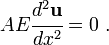
- Integrate twice to get the homogeneous solution

Particular solution.
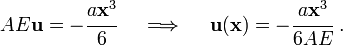
- The ODE is
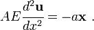
- Integrate twice to get the particular solution (and assume that the constants of integration are zero)
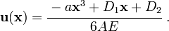
General solution.
- Add the homogeneous and particular parts to get
Apply BCs.
- At , . Therefore,
 .
. - At ,

Solution.
- The displacement field in the bar is

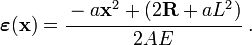
- The strain in the bar is
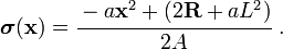
- The stress in the bar is
A plot of this solution is shown in Figure 2. All known quantities have been taken to be 1 for the plot.
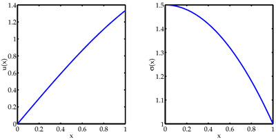 Figure 2. Exact solution for the axial loading of a bar. |