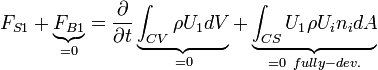
Fluid Mechanics for MAP/Analytical solutions of internal and external flows
< Fluid Mechanics for MAP>back to Chapters of Fluid Mechanics for MAP
>back to Chapters of Microfluid Mechanics
Internal and External Incompressible Viscous Flows
|
Flows completely bounded by solid surfaces are called internal flows. External flows are flows over bodies immersed in an unbounded fluid[1]. Internal flows might be laminar or turbulent. The state of the flow regime is dependent on Re. There might be an analytical solution for laminar flows but not for turbulent flows. 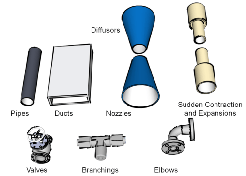 Flows through pipes, ducts, nozzles, diffusers, valves and fittings are examples of internal flows. |
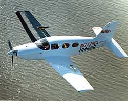 Flow around an aircraft is classified under external flows. 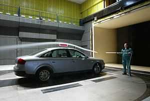 Flow around a car is classified under external flows. |
Laminar and Turbulent Channel and Pipe flows
|
At fully developed state the velocity profile becomes parabolic for laminar flow. The average velocity at any cross section is:  For the same flow value i.e. The reason is the turbulent eddies, which causes more momentum loss to the wall i.e. higher velocity gradients close to the wall. Note that such a direct comparison is only valid at the same |
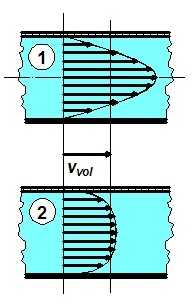 Velocity profiles for laminar (upper) and turbulent (lower) states at the same mass flow rate |
 , the fully developed turbulent pipe flow, would have higher velocity close to the wall and lower velocity at the center.
 .
.|
|
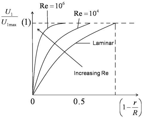 Development of velocity profile in a pipe with increasing Reynolds number |
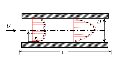
Concept of Fully Developed Flow
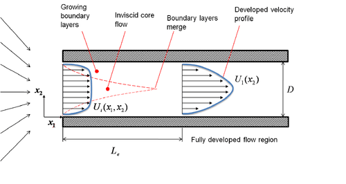
Consider the flow in a channel between two plates having a height of  and an infinite depth in
  direction.
Starting from the entrance, the boundary layers develop due to the no-slip condition on the wall.
At a finite distance, the boundary layers merge and the inviscid core (field with no velocity gradient in
direction.
Starting from the entrance, the boundary layers develop due to the no-slip condition on the wall.
At a finite distance, the boundary layers merge and the inviscid core (field with no velocity gradient in  direction) vanishes.
The flow becomes fully viscous. The velocity field in
direction) vanishes.
The flow becomes fully viscous. The velocity field in  direction adjusts slightly further until
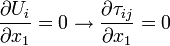
  and it no longer changes with direction. This state of the flow is called fully-developed. At that state:
Because of the two-dimensional nature of the flow, no gradient of the velocity quantities in direction is expected starting from the entrance.
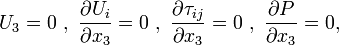
Hence,

The entrance lengths for laminar pipe and channel flows are, respectively[4]:
![\frac{Le_{pipe}}{D} = \left[(0.619)^{1.6} + (0.0567Re)^{1.6}\right]^{\frac{1}{1.6}}](../I/m/07b7e37a7bf918da5c876dbe0c763df5.png)
![\frac{Le_{channel}}{D} = \left[(0.631)^{1.6} + (0.0442Re)^{1.6}\right]^{\frac{1}{1.6}}](../I/m/38520f6a449dc2b001494b700126a5ed.png)
Fully Developed Laminar Flow Between Infinite Parallel Plates
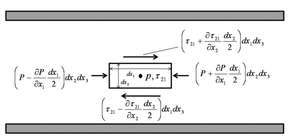
Consider the fully developed laminar flow between two infinite plates.
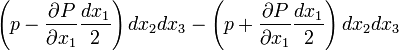
Consider the continuity equation and momentum equation in direction for an incompressible steady flow between two infinite plates as shown.
Continuity Equation
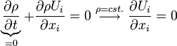
Since  ,
,  because it is a fully-developed and two dimensional flow. Hence,
  reads
reads
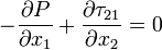
As is zero on the walls, it should be zero in the whole fully developed region, i.e.

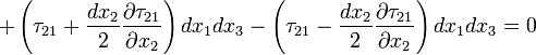
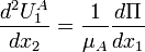
Momentum Equation in j-direction
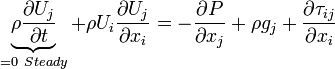
in direction ,
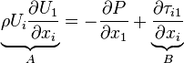
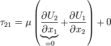
Consider term A:
![\rho U_{i}\frac{\partial U_{1}}{\partial x_{i}} = \rho \left[U_{1}\underbrace{\frac{\partial U_{1}}{\partial x_{1}}}_{= 0\ Fully-developed} + \underbrace{U_{2}}_{= 0}\frac{\partial U_{1}}{\partial x_{2}} + \underbrace{U_{3}}_{=0\ fully-developed\ 2D }\underbrace{\frac{\partial U_{1}}{\partial x_{3}}}_{= 0\ 2D}\right]=0](../I/m/bea4ea655220101738dfd02073d63de4.png)
Consider term B:
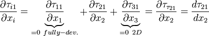
hence  .
.
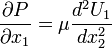
Thus the momentum equation in direction reads:
This equation should be valid for all and . This requires that  = constant.
Remember  is the stress in direction on a face normal to direction.
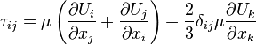
thus,
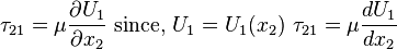
Thus the momentum equation reads:
This equation can be obtained also by using the Reynold's transport equations for a differential volume.
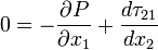
The momentum equation in direction,
The flux term becomes zero since for fully-developed flow incoming flux is equal to the outgoing flux. Thus,

That is:
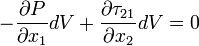
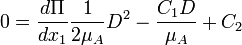
Finally, the governing equation of this kind of flow becomes:
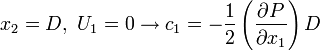
with the following boundary conditions:
 and
and 
Integrating the equation once results in a linear function of :
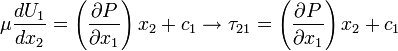
The second integration reads:
The integration constants is obtained by using the boundary conditions:

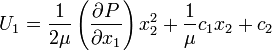
Finally, the velocity profile reads:
![\begin{array}{lll}
U_{1} &=& \frac{1}{2\mu}\left(\frac{\partial P}{\partial x_{1}}x_{2}^{2}\right) - \frac{1}{2\mu}\left(\frac{\partial P}{\partial x_{1}}\right)D{x_{2}}\\
&=&\frac{D^{2}}{2\mu}\left(\frac{\partial P}{\partial x_1}\right) \left[\left(\frac{x_{2}}{D}\right)^{2} - \left(\frac{x_{2}}{D}\right)\right]
\end{array}](../I/m/67f2d55d01ae818c748b5731424227b2.png)
Note that the velocity profile is parabolic!
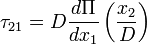
The shear stress becomes:
![\begin{array}{lll}
\tau_{21} &=& \left(\frac{\partial P}{\partial x_{1}}\right)x_{2} - \frac{1}{2}\left(\frac{\partial P}{\partial x_{1}}\right)D \\
&=& D\left(\frac{\partial P}{\partial x_{1}}\right)\left[\frac{x_{2}}{D} - \frac{1}{2}\right]
\end{array}](../I/m/c57c57ddcfce3639ec7f7bdf9e7db3c6.png)
at the wall i.e. at = 0 and = D
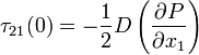
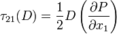
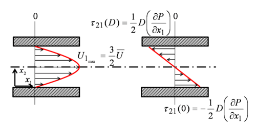
Note that is maximum near the wall, i.e. momentum loss is maximum near the wall. This is due to the maximum velocity gradient  near the wall!
The volume flow rate is,
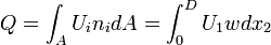
where  is the depth of the channel.
Thus the volume flow rate per depth is given by:
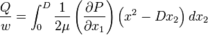
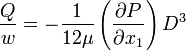
Note that  should be constant for the fully developed flow. Hence, for a channel with a finite length
  :
:
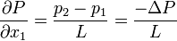
Where  is the pressure drop along L.
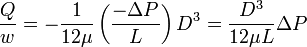
or the pressure drop can be calculated from:
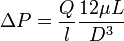
For the same flow rate, increasing the height of the channel would cause a drastic reduction in the pressure drop.
The average velocity  is:
is:

The maximum velocity occurs when:
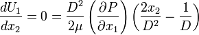
Hence, at  ,
, 
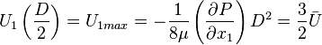
The velocity profile can be written as functions of bulk velocity  or maximum velocity
  by replacing their value the velocity profile equation:
![\begin{array}{lll}
U_{1} &=& -4 U_{1max} \left[\left(\frac{x_{2}}{D}\right)^{2} - \left(\frac{x_{2}}{D}\right)\right]\\
&=&-6 \overline{U} \left[\left(\frac{x_{2}}{D}\right)^{2} - \left(\frac{x_{2}}{D}\right)\right]
\end{array}](../I/m/9a93b081dd6a34df7183cad36795e592.png)
Same problem can be solved by using moving plates.
Example
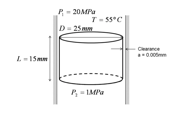
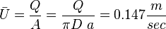
Consider the hydrolic control valve coprising a piston, fitted to a cylinder with a mean radial clearance of 0,005mm. Determine the leakage flow rate. The fluid is SAE low oil ( = 932
= 932  ,
,  =0.018
  at 55ºC). The flow can be assumed to be laminar, steady, incompressible, fully-developed flow.
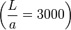
Since  = 5000 the flow in the clearance can be accepted to be 2-D, with the depth
  , thus:


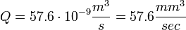
Check the Reynolds number to ensure that laminar flow assumption is correct.
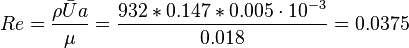
Re  , i. e. the flow is laminar.
Layered Channel Flow
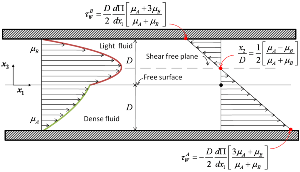
This channel flow contains two different and non miscible fluids. Fluids A and B flow at the same time through a channel, which is bounded two flat plates. They both occupy the half height of the channel. The fluid A has a viscosity  , a density
  and the mass flow
  . Fluid B, which is located above fluid A, has a viscosity
  , a density
  and the mass flow
  . The following differential equations correspond to the molecular momentum
  for each Fluid.
 and
and  .
.
With  yields the velocity field:
 and
and 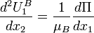
After integration of both equations we obtain:
 and
and 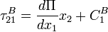
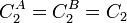
As boundary condition we consider that shear stress on the interface between A and B is the same. Therefore we obtain:
Then,
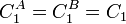
After the integration for the velocity field:
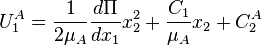
and
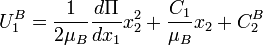
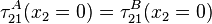
The second boundary condition turns out to be on the interface:
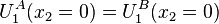 , i.e.
therefore,
 . The integration constants can be calculated with the following boundary conditions:
At 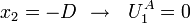 :
:
At 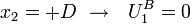 :
:
Therefore we obtain for the velocity distribution in the fluids A and B:
![U_{1}^{A} = -\frac{D^{2}}{2\mu_{A}}\frac{d\Pi}{dx_{1}} \left[+\frac{2\mu_{A}}{(\mu_{A} + \mu_{B})} + \left(\frac{\mu_{A} - \mu_{B}}{\mu_{A}+ \mu_{B}}\right)\left(\frac{x_{2}}{D}\right) - \left(\frac{x_{2}}{D}\right)^{2}\right] \ \ \ \ \](../I/m/d63de477ba7a2c6622fd8bade0c99726.png)
and
![U_{1}^{B} = -\frac{D^{2}}{2\mu_{B}}\frac{d\Pi}{dx_{1}} \left[+\frac{2\mu_{B}}{(\mu_{A} + \mu_{B})} + \left(\frac{\mu_{A} - \mu_{B}}{\mu_{A}+ \mu_{B}}\right)\left(\frac{x_{2}}{D}\right) - \left(\frac{x_{2}}{D}\right)^{2}\right]](../I/m/3acc9981f22a3ad89273f0cd50f3a243.png)
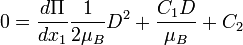
For the distribution of the shear stress we get:
![\tau_{21} = D\frac{d\Pi}{dx_{1}}\left[\left(\frac{x_{2}}{D}\right) - \frac{1}{2} \left(\frac{\mu_{A} - \mu_{B}}{\mu_{A}+ \mu_{B}}\right)\right]](../I/m/dca4190b800bf5c6f422a3c9fb2ca665.png)
If we choose  ,
,
![U_{1} = \frac{-D^{2}}{2\mu_{A}}\frac{d\Pi}{dx_{1}}\left[1 - \left(\frac{x_{2}}{D}\right)^{2}\right]](../I/m/95ed56492c59f79131e00d70d78dafbc.png)
The solution gives that of the channel flow. In other words, velocity has a parabolic profile with the peak in the middle of the channel and a linear shear stress distribution , where  at the channel's centerline.
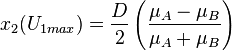
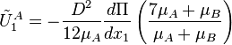
If  , the position where the maximal velocity occurs can be calculated by introducing on the velocity profile equation:
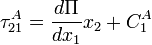
The shear stress on the upper plate is:
![\tau_{W}^{B} = \frac{D}{2}\frac{d\Pi}{dx_{1}}\left[\frac{\mu_{A} + 3\mu_{B}}{\mu_{A} + \mu_{B}}\right]](../I/m/69db437e48bde514a6d8a7cd74b4e6fa.png)
and the shear stress on the lower plate reads:
![\tau_{W}^{A} = -\frac{D}{2}\frac{d\Pi}{dx_{1}}\left[\frac{3\mu_{A} + \mu_{B}}{\mu_{A} + \mu_{B}}\right]](../I/m/2d04cf94d5ee398792c8da8c70854dc4.png)
The average velocities of the fluids A and B are:
and
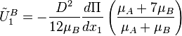
Hence the respectively mass flow rates are:
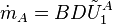
and
Navier Stokes Equation in Cyclindrical Coordinates
A change of variables on the Cartesian equations will yield[5] the following equations of momentum in r,  , and z directions:
![r:\;\;\rho \left(\frac{\partial u_r}{\partial t} + u_r \frac{\partial u_r}{\partial r} + \frac{u_{\phi}}{r} \frac{\partial u_r}{\partial \phi} + u_x \frac{\partial u_r}{\partial x} - \frac{u_{\phi}^2}{r}\right) =
-\frac{\partial p}{\partial r} +
\mu \left[\frac{1}{r}\frac{\partial}{\partial r}\left(r \frac{\partial u_r}{\partial r}\right) + \frac{1}{r^2}\frac{\partial^2 u_r}{\partial \phi^2} + \frac{\partial^2 u_r}{\partial x^2}-\frac{u_r}{r^2}-\frac{2}{r^2}\frac{\partial u_\phi}{\partial \phi} \right] + \rho g_r](../I/m/326d8e07ddc1526a1cd70104233cadd6.png)
![\phi:\;\;\rho \left(\frac{\partial u_{\phi}}{\partial t} + u_r \frac{\partial u_{\phi}}{\partial r} + \frac{u_{\phi}}{r} \frac{\partial u_{\phi}}{\partial \phi} + u_x \frac{\partial u_{\phi}}{\partial x} + \frac{u_r u_{\phi}}{r}\right) =
-\frac{1}{r}\frac{\partial p}{\partial \phi} +
\mu \left[\frac{1}{r}\frac{\partial}{\partial r}\left(r \frac{\partial u_{\phi}}{\partial r}\right) + \frac{1}{r^2}\frac{\partial^2 u_{\phi}}{\partial \phi^2} + \frac{\partial^2 u_{\phi}}{\partial z^2} + \frac{2}{r^2}\frac{\partial u_r}{\partial \phi} - \frac{u_{\phi}}{r^2}\right] + \rho g_{\phi}](../I/m/83005f646a4cf900917c729d44069769.png)
![x:\;\;\rho \left(\frac{\partial u_x}{\partial t} + u_r \frac{\partial u_x}{\partial r} + \frac{u_{\phi}}{r} \frac{\partial u_x}{\partial \phi} + u_x \frac{\partial u_x}{\partial x}\right) =
-\frac{\partial p}{\partial x} + \mu \left[\frac{1}{r}\frac{\partial}{\partial r}\left(r \frac{\partial u_x}{\partial r}\right) + \frac{1}{r^2}\frac{\partial^2 u_x}{\partial \phi^2} + \frac{\partial^2 u_x}{\partial x^2}\right] + \rho g_x.](../I/m/c06d898a0537c0c6772a89139322d4e2.png)
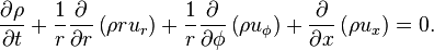
The continuity equation is:
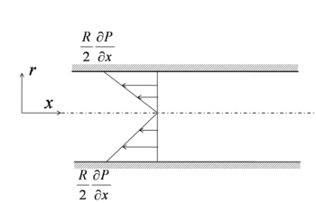
Fully Developed Pipe Flow
It is possible to use the same mathematical treatment like before to find and understand the velocity profile for fully developed flow inside a pipe with diameter D and infinite length. To show the flexibility, the same solution for this problem will be approached via 3 different ways.
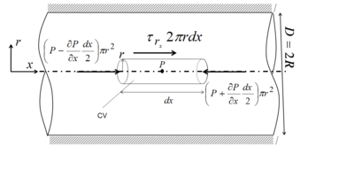
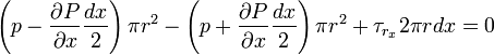
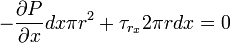
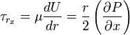
(i) Infinitesimal Cylinder at the center of the pipe
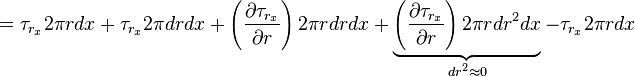
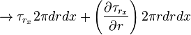
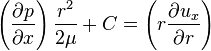
Applying the RTT to the infinitesimal cylindrical CV along the symmetry axis of horizontal pipe, in which the flow is fully developed, the conservation of mass and the transport side of the conservation of momentum equation drops. Only remaining term governing this kind of flow is the balance of the forces on the CV in  direction.

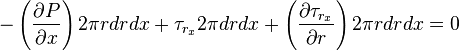
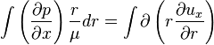
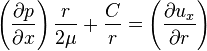
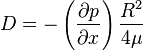
(ii) Infinitesimal thin hollow cylinder at the center
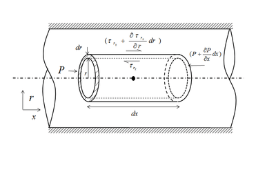
This time the pressure and viscous force is considered for a concentric hollow cylinder with radius of R and infinitesimally small thickness dr and length dx(as shown in the image besides) along x-direction. Considering pressure term on the cross-section of cylinder
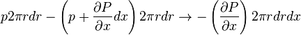
considering viscous shear stress on the surface of the cylinder
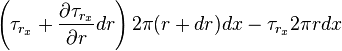
combining both term,we get the balance equation,
it could be rewritten as
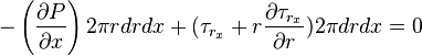
dividing both side with  ,we get
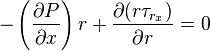
or,
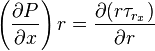
integrating both side ,
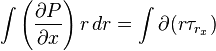
or,
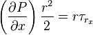
or,
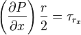
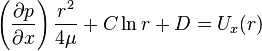
However,in a laminar flow!
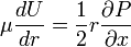
integrating,
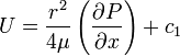
The boundary condition is:
Thus  can be calculated from the boundary condition.
or
![U = -\frac{R^{2}}{4\mu}\left(\frac{\partial P}{\partial x}\right)\left[1 - \left(\frac{r}{R}\right)^{2}\right]](../I/m/5822462a5d05bffb19f775385fa701c9.png)
(iii) Using NS in cylindrical co-ordinates:
![x:\rho \left(\underbrace{\frac{\partial u_x}{\partial t}}_{steady state} + \underbrace{u_r \frac{\partial u_x}{\partial r}}_{u_r=0} + \underbrace{\frac{u_{\phi}}{r} \frac{\partial u_x}{\partial \phi}}_{u_{\phi}=0}+\underbrace {u_x \frac{\partial u_x}{\partial x}}_{\frac{\partial u_x}{\partial x} =0}\right) =
-\frac{\partial p}{\partial x} + \mu \left[\frac{1}{r}\frac{\partial}{\partial r}\left(r \frac{\partial u_x}{\partial r}\right) +
\underbrace{\frac{1}{r^2}\frac{\partial^2 u_x}{\partial \phi^2}}_{=0} + \underbrace{\frac{\partial^2 u_x}{\partial x^2}}_{=0}\right] + \underbrace{\rho g_x}_{g_x=0}](../I/m/2703943825b95a12037729bfe2c70d64.png)
thus,
![\frac{\partial p}{\partial x} = \mu \left[\frac{1}{r}\frac{\partial}{\partial r}\left(r \frac{\partial u_x}{\partial r}\right)\right]](../I/m/8ea3d25ab25f3e03d3a0dce7ac947e2d.png)
or,
![\frac{\partial p}{\partial x} = \frac{\mu}{r}\left[\frac{\partial}{\partial r}\left(r \frac{\partial u_x}{\partial r}\right)\right]](../I/m/b00cef4d9a88397979ef7d13ed58be61.png)
or,
![\left(\frac{\partial p}{\partial x}\right)\frac{r}{\mu} = \left[\frac{\partial}{\partial r}\left(r \frac{\partial u_x}{\partial r}\right)\right]](../I/m/5c891326ef8fcac52266ee90ac3bb523.png)
Now, integrating both side with respect to  , we get
then,
dividing by r in both side , we get then
integrating again with respect to gives ,
Consequently, when  then
then  and
and  , as a result C=0.
On the other hand, when  then
then  , so
, so
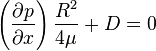
or,
By putting D to the primitive equation, we get,
Knowing the velocity profile we can evaluate relevant quantities. The shear stress profile will look like:
at r = 0 
at r = R 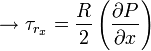
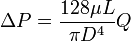
The volume flow rate would read
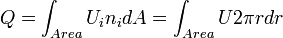
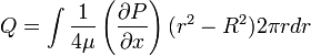
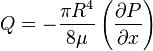
When we approximate 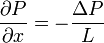
![Q = -\frac{\pi R^{4}}{8\mu}\left[\frac{-\Delta P}{L}\right] = \frac{\pi \Delta PR^{4}}{8\mu L} = \frac{\pi \Delta PD^{4}}{128\mu L}](../I/m/b4d91fd845cf33eea2d2fdc95ed07c75.png)
Increase radius to create drastic reduction in the pressure drop.
The mean velocity is:
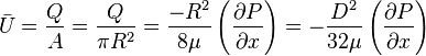
The location where maximum velocity occurs can be found be setting:
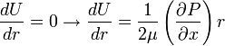
at r = 0  U =
U =  .
.
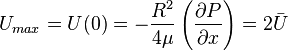
Note that in a channel was  .
.
 can be written as a function of i.e.
![U = \underbrace{-\frac{R^{2}}{4\mu}\left(\frac{\partial P}{\partial x}\right)}_{U_{max}}\left[1 - \left(\frac{r}{R}\right)^{2}\right]](../I/m/8a1849fc481709abd71938be1d170c54.png)
![\frac{U}{U_{max}} = \left[1 - \left(\frac{r}{R}\right)^{2}\right]](../I/m/c998dfd83829d0032b46b635180bb941.png)
Again, the velocity profile becomes parabolic.
References
- ↑ Fox, R.W. and McDonald, A.T., “Introduction to Fluid Mechanics”, John Willey and Sons.
- ↑ M. Nishi. PhD Thesis Friedrich-Alexander-Universität Erlangen-Nürnberg, 2009.
- ↑ M. Nishi, B. Ünsal, F. Durst, and G. Biswas. J. Fluid Mech., 614:425–446, 2008.
- ↑ Durst, F., Ray, S., Unsal, B., and Bayoumi, O. A., 2005, “The Development Lengths of Laminar Pipe and Channel Flows,” J. Fluids Eng., 127, pp. 1154– 1160.
- ↑ Acheson, D.J.: Elementary fluid dynamics, Clarendon Press, 1990.