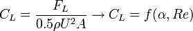
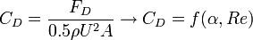
Fluid Mechanics for MAP/Dimensional Analysis

< Fluid Mechanics for MAP

>back to Chapters of Fluid Mechanics for MAP

>back to Chapters of Microfluid Mechanics

Motivation

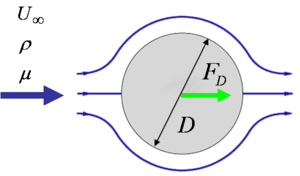
Consider the steady flow around a submerged sphere. Say we are interested in the drag force on the sphere.

F_D=f(U_\infty, D, \rho, \mu)

Let's say 10Bold text measurement points are enough for one curve, which shows the effect of one parameter while keeping the others constant. In order to monitor the effect of all variables, $10^4$ separate measurements are needed. When each measurement takes 1/2 hr, all test series need 2.5 years.

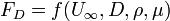
By using dimensional analysis, we can reduce $F_D$ to an equivalent form:

\frac{F_D}{\rho U_\infty^2 D^2}=g\left(\frac{\rho U_\infty D}{\mu}\right)\ \ \ \text{or commonly written as} \ \ \ \underbrace{C_D}_{Drag\ coefficient}= \underbrace{g\left(\frac{\rho U_\infty D}{\mu}\right)}_{Reynolds\ number}

Both sides are dimensionless. Function $g$ is different than $f$ but it contains all necessary information.

Full scale models might be impossible or prohibitively expensive. There might be numerous number of parameters to be tested.

Figure:Commercial Aircraft

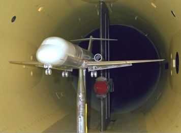Figure:Model flight in windtunnel

Under which conditions these tests are realistic? Are the both flows dynamically similar?

“Dimensional analysis is a method which reduces number and complexity of experimental variables which affect a given physical phenomenon, using a sort of compacting technique.” (White 1979)

Dimensional analysis (DA) helps us to formulate dimensionless forms of governing equations and simplify them by the determination insignificant terms:

\rho\left[\frac{\partial U_{j}}{\partial t} + U_{i}\frac{\partial U_{j}}{\partial x_{i}}\right] = -\frac{\partial P}{\partial x_{j}} + \frac{\partial}{\partial x_{i}}\left[\mu\left(\frac{\partial U_{j}}{\partial x_{i}} + \frac{\partial U_{i}}{\partial x_{j}}\right) - \frac{2}{3} \delta_{ij}\mu \frac{\partial U_{k}}{\partial x_{k}}\right]\rho g_{j}

\rho^{*}\left[St\frac{\partial U_{j}^{*}}{\partial t^{*}} + U^{*}_{i}\frac{\partial U_{j}^{*}}{\partial x_{i}^{*}}\right] = -Eu\frac{\partial P^{*}}{\partial x_{j}^{*}} + \frac{1}{Re}\frac{\partial}{\partial x^{*}_{i}}\left[\mu^{*}\left(\frac{\partial U^{*}_{j}}{\partial x^{*}_{i}} + \frac{\partial U_{i}^{*}}{\partial x^{*}_{j}}\right) - \frac{2}{3}\delta_{ij}\mu^{*}\frac{\partial U_{k}^{*}}{\partial x_{k}^{*}}\right] + \frac{1}{Fr}\rho^{*}g_{j}^{*}

\rho^{*} \left[St\frac{\partial U^{*}_{j}}{\partial t^{*}} + U_{i}^{*}\frac{\partial U^{*}_{j}}{\partial x^{*}_{i}}\right] = -\frac{\partial P^{*}}{\partial x^{*}_{j}}

This is the non-dimensional form of Euler equation.

Benefits of dimensional analysis (DA)

One obvious goal of our efforts should be to obtain the most information from the fewest experiments. Dimensional analysis (DA) is an important tool that often helps us to achieve this goal.

The benefits of this dimensionless representation are:

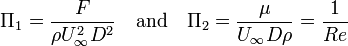
We do not have to vary each variable: It is enough that we vary only Re and measure CD. As a result, we have enormous time and money saving.
Dimensional analysis (DA) provides “scaling laws” which can convert data from a cheap small model to provide information about an expensive large prototype.
DA helps our thinking and planning of an experiment or a theory.
- It suggests dimensionless ways of writing equations.
- One can find variables which can be discarded.

As a result, we can avoid to waste money and time while we use experimental and computational resources.

Derivation of dimensionless numbers

Buckingham Π theorem provides a method for computing sets of dimensionless numbers from the given variables, even if the form of the equation is still unknown.

Consider the steady flow around a sphere, which shows no separation. We will find out the dimensionless numbers governing this flow:

Step 1: List all the parameters involved. Let $n$ be the number of parameters.

F_D, U_\infty, D, \rho, \mu \ \rightarrow \ \ n=5

Step 2: Select a set of primary dimensions, e.g. $M L tT q$ (mass, length, time, temperature, elec. charge or $FLtTq$ (Force, length, ...).

M,L\ \text{and}\ t\ \ \ \text{are selected to be the primary dimensions.}

Step 3: List the dimensions of all parameters. Let $r$ be the number of primary dimensions.

F,\ U_\infty,\ D,\ \rho,\ \mu \ \ \rightarrow\ \ \frac{ML}{t^2},\ \frac{L}{t},\ L,\ \frac{M}{L^3},\ \frac{M}{Lt}\ \ \ \ \rightarrow \ \ r=3\ \text{primary dimensions}

Step 4: Select $r$ number of parameters, including all the primary dimensions. No two parameters should have the same net dimension differing by only a single exponent: for example do not include both $L$ and $L^4$ .

U_\infty,\ D,\ \rho \ \ \rightarrow \ \ m = r = 3 \ \ \text{repeating parameters}

Step 5: Set up dimensional equations combining the parameters selected in Step 4 with each of the other parameters in turn to form $n-m$ dimensionless groups.

$n-m=2$ dimensionless groups will result. The dimensional equations are:

\Pi_1\ =\ U_\infty^aD^b\rho^cF= \left(\frac{L}{t}\right)^a \left(L\right)^b \left(\frac{M}{L^3}\right)^c\left(\frac{ML}{t^2}\right)=M^0L^0t^0

\Pi_2\ =\ U_\infty^dD^e\rho^f\mu= \left(\frac{L}{t}\right)^d \left(L\right)^e \left(\frac{M}{L^3}\right)^f\left(\frac{M}{Lt}\right)=M^0L^0t^0

solving above equations delivers $a=-2,b=-2,c=-1,d=-1,e=-1\ \text{and}\ f=-1$ . Hence

\Pi_1=\frac{F}{\rho U_\infty^2 D^2}\ \ \ \text{and}\ \ \ \Pi_2=\frac{\mu}{U_\infty D \rho}=\frac{1}{Re}

The functional relationship $\Pi_1=f(\Pi_2)$ should be determined experimentally and/or numerically.

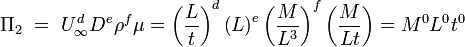
Application examples of non-dimensional numbers

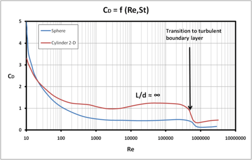
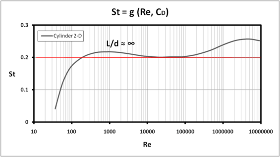
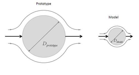
Flow around a cylinder and a sphere

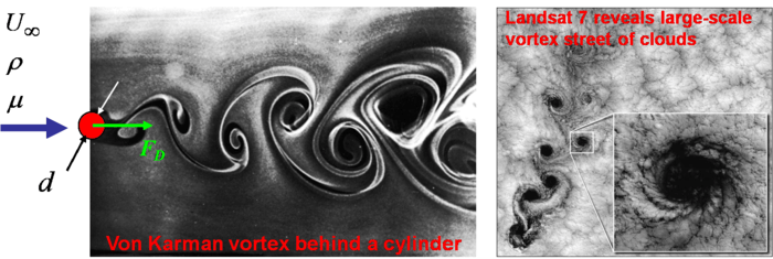
In a very large Re range the wake is unsteady, quasi time-periodic.

Important dimensionless numbers are:

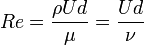$Re = \frac{\rho U d}{\mu} = \frac{U d}{\nu}$ where $\nu = \frac{\mu}{\rho}$ is the kinematik viscosity.

$St = \frac{f d}{U} = \frac{w d}{2\pi U}$ where f is the dominant frequency of the wake structures.

$C_{D} = \frac{F_{D}}{0.5\rho U^{2}A}$ where A is the projected area to the flow.

$\frac{L}{d}$ is also important for flow around a cylinder.

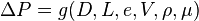
Losses in pipe flows

The pressure drop along the pipe can be written as:

$\ \Delta P = g(D,L,e,V,\rho,\mu)$ where $\ e$ is the average height of surface roughness and V is the average velocity.

\ \zeta=\frac{\Delta P}{0.5\rho V^{2}} = \Phi \left(Re,\frac{L}{D},\frac{e}{D}\right) \rightarrow \zeta= \frac{L}{D}f\left(Re, \frac{e}{D}\right)

where $\ f$ is the friction factor.

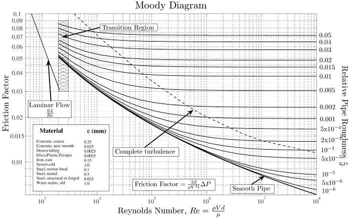Moody diagram

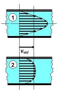Velocity profiles for laminar (upper) and turbulent (lower) states at the same mass flow rate

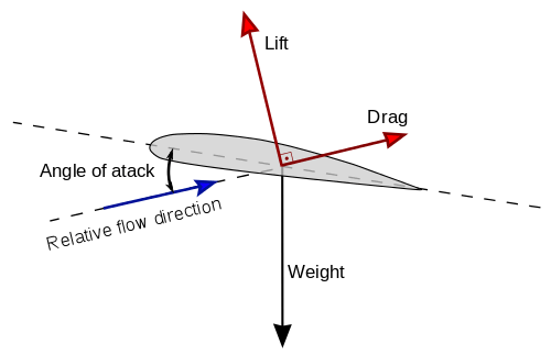
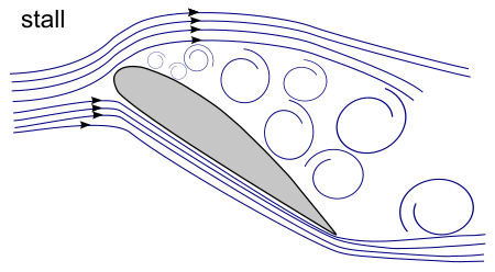
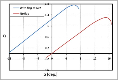
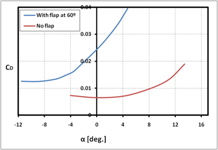
Lift and drag forces on airfoils

C_{L} = \frac{F_{L}}{0.5 \rho U^{2}A} \rightarrow C_{L} = f(\alpha,Re)

C_{D} = \frac{F_{D}}{0.5 \rho U^{2}A} \rightarrow C_{D} = f(\alpha,Re)

Non-dimensionalization of Governing Equations

An isothermal and newtonian fluid flow is governed by the following equations

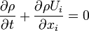
Conservation of Mass (continuity equation):

\frac{\partial \rho}{\partial t} +\frac{\partial \rho U_{i}}{\partial x_{i}} = 0

Conservation of Momentum

\rho\left[\frac{\partial U_{j}}{\partial t} + U_{i}\frac{\partial U_{j}}{\partial x_{i}}\right] = -\frac{\partial P}{\partial x_{j}} + \frac{\partial}{\partial x_{i}}\left[\mu\left(\frac{\partial U_{j}}{\partial x_{i}} + \frac{\partial U_{i}}{\partial x_{j}}\right) - \frac{2}{3} \delta_{ij}\mu \frac{\partial U_{k}}{\partial x_{k}}\right]\rho g_{j}

One can normalize each variable with a characteristic parameter, which has the same dimension

\ x_{i} = L_{c}x_{i}^{*}\ ,t = t_{c}t^{*}\ ,U_{j} = U_{c}U^{*}_{j}\ ,\ \rho = \rho_{c}\rho^{*}\ ,\ g_{j} = g_{c}g^{*}_{j}\ ,\ \mu = \mu_{c}\mu^{*}\ ,\ P=\Delta P_{c}P^{*}

Inserting these into the continuity equation

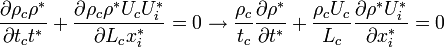
\frac{\partial \rho_{c}\rho^{*}}{\partial t_{c}t^{*}} + \frac{\partial \rho_{c}\rho^{*}U_{c}U^{*}_{i}}{\partial L_{c}x^{*}_{i}} = 0 \rightarrow \frac{\rho_{c}}{t_{c}}\frac{\partial \rho^{*}}{\partial t^{*}} + \frac{\rho_{c}U_{c}}{L_{c}}\frac{\partial \rho^{*}U_{i}^{*}}{\partial x^{*}_{i}} = 0

Dividing by $\frac{\rho_{c}U_{c}}{L_{c}}$

\underbrace{\frac{L_{c}}{t_{c}U_{c}}}_{St}\frac{\partial \rho^{*}}{\partial t^{*}} + \frac{\partial \rho^{*}U_{i}^{*}}{\partial x_{i}^{*}} = 0

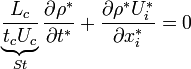
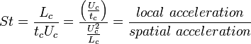
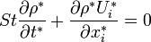
where St: Strouhal Number

St=\frac{L_{c}}{t_{c}U_{c}} = \frac{\left(\frac{U_{c}}{t_{c}}\right)}{\frac{U_{c}^{2}}{L_{c}}} = \frac{local\ acceleration}{spatial\ acceleration}

Similarly, we can apply this technique to make the momentum equation non-dimensional:

\rho_{c}\rho^{*}\left[\frac{U_{c}}{t_{c}}\frac{\partial U_{j}^{*}}{\partial t^{*}} + \frac{U_{c}^{2}}{L_{c}}U_{i}^{*}\frac{\partial U_{j}^{*}}{\partial x^{*}_{i}}\right] = -\frac{\Delta P_{c}}{L_{c}}\frac{\partial P^{*}}{\partial x_{j}^{*}} + \frac{\mu_{c}U_{c}}{L_{c}^{2}}\frac{\partial}{\partial x_{i}^{*}}\left[\mu^{*}\left(\frac{\partial U_{j}^{*}}{\partial x_{i}^{*}} + \frac{\partial U_{i}^{*}}{\partial x_{j}^{*}}\right) - \frac{2}{3}\delta_{ij}\mu^{*} \frac{\partial U_{k}^{*}}{\partial x_{k}^{*}}\right] + \rho_{c}g_{c}\rho^{*}g^{*}_{j}

Dividing by $\frac{\rho_{c}U_{c}^{2}}{L_{c}}$

\rho^{*}\left[\underbrace{\frac{L_{c}}{t_{c}U_{c}}}_{St}\frac{\partial U_{j}^{*}}{\partial t^{*}} + U_{i}^{*}\frac{\partial U_{j}^{*}}{\partial x^{*}_{i}}\right] = \underbrace{-\frac{\Delta P_{c}}{\rho_{c}U_{c}^{2}}}_{Eu}\frac{\partial P^{*}}{\partial x_{j}^{*}} + \underbrace{\frac{\mu_{c}}{\rho_{c}U_{c}L_{c}}}_{\frac{1}{Re}}\frac{\partial}{\partial x_{i}^{*}}\left[\mu^{*}\left(\frac{\partial U_{j}^{*}}{\partial x_{i}^{*}} + \frac{\partial U_{i}^{*}}{\partial x_{j}^{*}}\right) - \frac{2}{3}\delta_{ij}\mu^{*} \frac{\partial U_{k}^{*}}{\partial x_{k}^{*}}\right] + \underbrace{\frac{g_{c}L_{c}}{U_{c}^{2}}}_{\frac{1}{Fr}}\rho^{*}g^{*}_{j}

Eu: Euler Number $=\frac{\Delta P_{c}}{\rho_{c}U_{c}^{2}} = \frac{static\ pressure}{dynamic\ pressure}$

Re: Reynolds Number 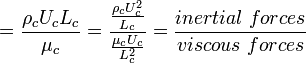$=\frac{\rho_{c}U_{c}L_{c}}{\mu_{c}} = \frac{\frac{\rho_{c}U_{c}^{2}}{L_{c}}}{\frac{\mu_{c}U_{c}}{L_{c}^{2}}} = \frac{inertial\ forces}{viscous\ forces}$

Fr: Froude Number 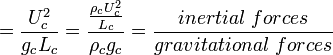$=\frac{U_{c}^{2}}{g_{c}L_{c}} = \frac{\frac{\rho_{c}U_{c}^{2}}{L_{c}}}{\rho_{c}g_{c}} = \frac{inertial\ forces}{gravitational\ forces}$

The resulting dimensionless conservation of mass and of momentum equations are:

St\frac{\partial \rho^{*}}{\partial t^{*}} + \frac{\partial \rho^{*}U_{i}^{*}}{\partial x_{i}^{*}} = 0

\rho^{*}\left[St\frac{\partial U_{j}^{*}}{\partial t^{*}} + U_{i}^{*}\frac{\partial U_{j}^{*}}{\partial x^{*}_{i}}\right] = -Eu\frac{\partial P^{*}}{\partial x_{j}^{*}} + \frac{1}{Re}\frac{\partial}{\partial x_{i}^{*}}\left[\mu^{*}\left(\frac{\partial U_{j}^{*}}{\partial x_{i}^{*}} + \frac{\partial U_{i}^{*}}{\partial x_{j}^{*}}\right) - \frac{2}{3}\delta_{ij}\mu^{*} \frac{\partial U_{k}^{*}}{\partial x_{k}^{*}}\right] + \frac{1}{Fr}\rho^{*}g^{*}_{j}

These equation indicates that solution of similar problems for two problems, say A and B, can only be same when the dimensionless numbers are equal:

St_{A} = St_{B},\ Eu_{A} = Eu_{B},\ Re_{A} = Re_{B},\ Fr_{A} = Fr_{B}

Furthermore, we should warrant the similarity of the boundary conditions and this requires geometric similarity.

Selection of characteristic variables and Simplifications to governing equations

Consider the momentum transport equation:

\rho^{*}\left[St\frac{\partial U_{j}^{*}}{\partial t^{*}} + U_{i}^{*}\frac{\partial U_{j}^{*}}{\partial x^{*}_{i}}\right] = -Eu\frac{\partial P^{*}}{\partial x_{j}^{*}} + \frac{1}{Re}\frac{\partial}{\partial x_{i}^{*}}\left[\mu^{*}\left(\frac{\partial U_{j}^{*}}{\partial x_{i}^{*}} + \frac{\partial U_{i}^{*}}{\partial x_{j}^{*}}\right) - \frac{2}{3}\delta_{ij}\mu^{*} \frac{\partial U_{k}^{*}}{\partial x_{k}^{*}}\right] + \frac{1}{Fr}\rho^{*}g^{*}_{j}

For very low St, i.e. when tc < Uc/Lc, in other words when local acceleration much smaller than spatial acceleration, the flow can be accepted to be steady. Thus the first term at LHS can be neglected, i.e. the momentum equation reads

\rho^{*}U_{i}^{*}\frac{\partial U_{j}^{*}}{\partial x^{*}_{i}} = -Eu\frac{\partial P^{*}}{\partial x_{j}^{*}} + \frac{1}{Re}\frac{\partial}{\partial x_{i}^{*}}\left[\mu^{*}\left(\frac{\partial U_{j}^{*}}{\partial x_{i}^{*}} + \frac{\partial U_{i}^{*}}{\partial x_{j}^{*}}\right) - \frac{2}{3}\delta_{ij}\mu^{*} \frac{\partial U_{k}^{*}}{\partial x_{k}^{*}}\right] + \frac{1}{Fr}\rho^{*}g^{*}_{j}

When we select: 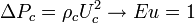$\Delta P_{c} = \rho_{c}U_{c}^{2} \rightarrow Eu = 1$

\rho^{*}\left[St\frac{\partial U_{j}^{*}}{\partial t^{*}} + U_{i}^{*}\frac{\partial U_{j}^{*}}{\partial x^{*}_{i}}\right] = -\frac{\partial P^{*}}{\partial x_{j}^{*}} + \frac{1}{Re}\frac{\partial}{\partial x_{i}^{*}}\left[\mu^{*}\left(\frac{\partial U_{j}^{*}}{\partial x_{i}^{*}} + \frac{\partial U_{i}^{*}}{\partial x_{j}^{*}}\right) - \frac{2}{3}\delta_{ij}\mu^{*} \frac{\partial U_{k}^{*}}{\partial x_{k}^{*}}\right] + \frac{1}{Fr}\rho^{*}g^{*}_{j}

In one phase flows, this kind of selection of the characteristic pressure is common. Thus, one can see that the pressure gradient can not be neglected.

For flows in which cavitation occurs, one can use the vapor pressure of the fluid in the characteristic pressure term:

$\Delta P_{c} = P - P_{v} \rightarrow Eu = Ca = Cavitation\ Number = \frac{P - P_{v}}{\rho_{c}U_{c}^{2}}$

\rho^{*}\left[St\frac{\partial U_{j}^{*}}{\partial t^{*}} + U_{i}^{*}\frac{\partial U_{j}^{*}}{\partial x^{*}_{i}}\right] = -Ca\frac{\partial P^{*}}{\partial x_{j}^{*}} + \frac{1}{Re}\frac{\partial}{\partial x_{i}^{*}}\left[\mu^{*}\left(\frac{\partial U_{j}^{*}}{\partial x_{i}^{*}} + \frac{\partial U_{i}^{*}}{\partial x_{j}^{*}}\right) - \frac{2}{3}\delta_{ij}\mu^{*} \frac{\partial U_{k}^{*}}{\partial x_{k}^{*}}\right] + \frac{1}{Fr}\rho^{*}g^{*}_{j}

The Froude number is important when gravity starts to play an important role, i.e. when buoyancy effects occurs due to density differences and, especially for multi-phase flows. For example, we deal with a two-phase flow, for which two fluids can be accepted to be immiscible, like water and air in the spill way of a dam. In order to introduce the effect of density into the Fr number, the characteristic gravity in the Fr number can be selected to be:

g_{c} = g \frac{\rho_{2} - \rho_{1}}{\rho_{2}}

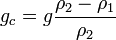where

\rho_{2}>\rho_{1} \rightarrow Fr = \left(\frac{1}{g(\rho_{2} - \rho_{1})}\right)\left(\frac{\rho_{2}U_{c}^{2}}{L_{c}}\right) = \frac{inertial\ forces}{bouyancy\ forces}

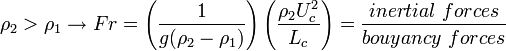
Thus, when the density difference becomes negligible, Fr becomes very large and the momentum equation reduces to:

\rho^{*}\left[St\frac{\partial U_{j}^{*}}{\partial t^{*}} + U_{i}^{*}\frac{\partial U_{j}^{*}}{\partial x^{*}_{i}}\right] = -Eu\frac{\partial P^{*}}{\partial x_{j}^{*}} + \frac{1}{Re}\frac{\partial}{\partial x_{i}^{*}}\left[\mu^{*}\left(\frac{\partial U_{j}^{*}}{\partial x_{i}^{*}} + \frac{\partial U_{i}^{*}}{\partial x_{j}^{*}}\right) - \frac{2}{3}\delta_{ij}\mu^{*} \frac{\partial U_{k}^{*}}{\partial x_{k}^{*}}\right]

The Froude number can be important also for one phase flows with large density gradients. In order to introduce this effect, the characteristic gravity in the Fr number can be written by using the density gradient:

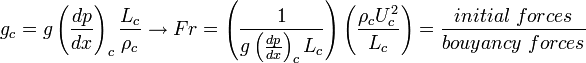
g_{c} = g\left(\frac{dp}{dx}\right)_{c} \frac{L_{c}}{\rho_{c}} \rightarrow Fr = \left(\frac{1}{g\left(\frac{dp}{dx}\right)_{c}L_{c}}\right)\left(\frac{\rho_{c}U_{c}^{2}}{L_{c}}\right) = \frac{initial\ forces}{bouyancy\ forces}

This form of the Fr number can be used in the field of convective heat transfer at which the characteristic velocities are very low such that buoyancy dominates the flow motion. In the mixing of fluids having different densities, this form can also be one of the important non-dimensional numbers.

Another simplification can be made: when the Re number of the flow is very high, the viscous stresses can be eliminated in regions where the velocity gradients are low. For example, for the cruising aircrafts the Re number is in the order of millions. Therefore, it is common approach, to use the inviscid form of Navier Stokes equations for flow simulations around cruising aircrafts, except in the vicinity of the aircraft body. For such a flow, we can neglect the gravitational effects, since Fr becomes very large. Moreover, Eu can be accepted to be 1 as shown before. Thus, the governing momentum equation reduces to the non-dimensional form of Euler equations:

\rho^{*}\left[St\frac{\partial U_{j}^{*}}{\partial t^{*}} + U_{i}^{*}\frac{\partial U_{j}^{*}}{\partial x^{*}_{i}}\right] = -\frac{\partial P^{*}}{\partial x_{j}^{*}}

Similarity considerations

Once the variables are selected and the dimensional analysis is performed, the experimenter seeks to achieve similarity between the model tested and the prototype to be designed.

Flow conditions for a model test are completely similar if all relevant dimensionless parameters $(\Pi_{1},\Pi_{2},...,\Pi_{n})$ have the same corresponding values for the model and the prototype (White):

\Pi_{1model} = \Pi_{1prototype}, \Pi_{2model} =\Pi_{2prototype},..., \Pi_{n\ model} = \Pi_{n\ prototype}

But this is easier said than done.

Instead of complete similarity, the engineering literature speaks of particular types of similarity:

Geometric similarity

Kinematic similarity

Dynamic similarity

Thermal similarity

Geometric similarity

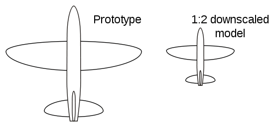
A model and a prototype are geometrically similar if and only if all body dimensions in all three coordinates have the same linear-scale ratio.

All angles are preserved in geometric similarity. All flow directions are preserved. The orientations of model and prototype with respect to the surroundings must be identical.

1:2 down-scaled aircraft model

Kinematic similarity

The motions of two systems are kinematically similar if homologous particles lie at homologous points at homologous times.

In other words, kinematic similarity requires that the model and prototype have dependent length-scale and time-scale ratios. This requires, for example, similarity in Re or Mach number. The result is that the velocity-scale ratio will be the same for both:

One exception, in which the length and the time-scales becomes independent is the frictionless low-speed flow, without any free-surface.

Frictionless low speed flow

$\displaystyle D_{model} = \alpha D_{prototype}$

and

$\displaystyle V_{model} = \beta V_{prototype}$

For a frictionless two-phase flow, the Froude numbers should be same, thus

From:

Fr_{model} = \frac{V^{2}_{model}}{gL_{model}} = \frac{V^{2}_{prototype}}{gL_{prototype}} = Fr_{prototype}

and,

L_{model} = \alpha L_{prototype} \rightarrow V_{model} = \sqrt{\alpha}V_{prototype}

we obtain:

\frac{L_{model}}{L_{protorype}} = \alpha

and,

\frac{T_{model}}{T_{prototype}} = \frac{L_{model}/V_{model}}{L_{prototype}/V_{prototype}} = \sqrt{\alpha}

Similarity consideration for wave effect modelling

Dynamic similarity

Dynamic similarity exists when the model and the prototype have the same length scale ratio, time-scale ratio, and force-scale (or mass-scale) ratio.

Mathematically, Newton’s law for any fluid particle requires that the sum of the pressure force, gravity force, and friction force equal the acceleration term, or inertia force:

\displaystyle F_{inertia} = F_{body} + F_{pressure} + F_{viscous}

The dynamic-similarity ensure that each of these forces will be in the same ratio and have equivalent directions between model and prototype.

Again geometric similarity is a first requirement. Then dynamic similarity exists, simultaneous with kinematic similarity, if the model and prototype force and pressure coefficients are identical. This is ensured if:

For compressible flow, the model and prototype Reynolds number and Mach number and specific-heat ratio are correspondingly equal.
For incompressible flow
- With no free surface: model and prototype Reynolds numbers are equal.
- With a free surface: model and prototype Reynolds number, Froude number, and (if necessary) Weber number and cavitation number are correspondingly equal.

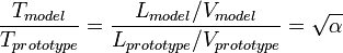
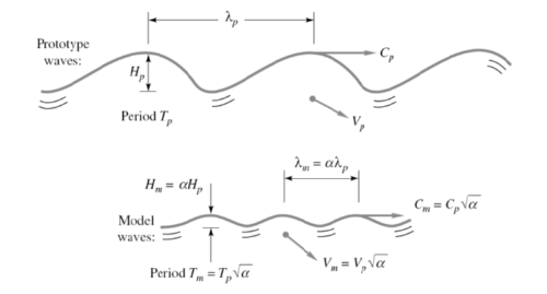
Incomplete similarity

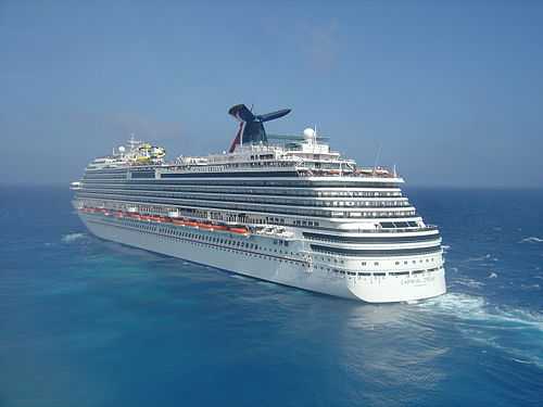
It is not possible to reach complete similarity in the laboratory for the wavy water flow around the ship

Not always, it is easy to obtain complete dynamic similarity.

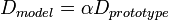
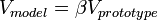
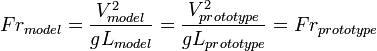
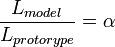
Consider the drag force on the surface of the ship shown. To have complete dynamic similarity between test model and prototype:

$Fr_{model} = Fr_{prototype},\ Re_{model} = Re_{prototype}$

For a 100 times downscaled test model, the Fr number similarity requires:

L_{model} = \frac{1}{100}L_{prototype} \rightarrow \frac{100V^{2}_{model}}{gL_{prototype}} = \frac{V^{2}_{prototype}}{gL_{prototype}} \rightarrow V_{model} = 10V_{prototype}

Thus, the Re number similarity can only be obtained at the same time

Re_{model} = \frac{V_{model}L_{model}}{\upsilon_{model}} = \frac{10V_{prototype}L_{prototype}}{\upsilon_{model}100} = \frac{U_{prototype}L_{prototype}}{\upsilon_{prototype}} = Re_{prototype}

$\rightarrow \upsilon_{model} = 0.1\upsilon_{prototype}$

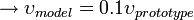
Only liquid which has less kinematic viscosity than water is mercury, and even with that fluid Re similarity can not be established. Since Froude number becomes more important than Re, in the experiments scaling is done using only Fr number.

An example study: Inhaler development

Flow Visualization in Inhalers: Inhaler in the Water Tunnel

Experimental setup

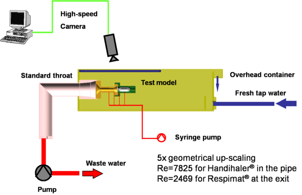
The flow in the Handihaler is unsteady. Thus, visualization is preferred in order to understand the flow character within the inhaler. The up-scaled models in water are used to slow down the speed of the flow so that we can record streaklines with a high-speed camera.

Flow in the Handihaler® and Respimat®

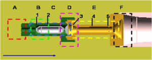
After preliminary visualization experiments, scenarios were planned. The flow region was divided into sub-regions. Dye injection holes were built in these sub-regions. Around 100 visualizations were made for original and modified geometries of Handihaler and Respimat.

The mechanism of particle discharge from the capsule is discovered.

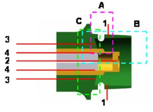
With the help of the prototypes we could easily study the effect of different flow and geometrical parameters on the unsteady flow within the Handihaler

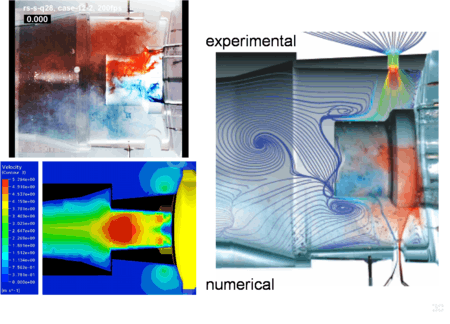
The visualization is used to validate numerical simulations.

Experiments versus simulations

Complete design of inhalers can be made by the utilization of non-dimensional numbers^[1].

Correlation between experiments and simulations

Conclusions

Dimensional analysis and similitude are two important tools in experimental research.

While analyzing a phenomenon one can use the dimensionless numbers to judge the importance of the governing effects.

Similarity considerations should be carefully performed to obtain useful results, especially when similarity is not complete.

Reference

↑ Int J Pharm. 2011 Sep 15;416(1):25-34. doi: 10.1016/j.ijpharm.2011.05.045. Epub 2011 Jun 28. A method for the aerodynamic design of dry powder inhalers. Ertunç O, Köksoy C, Wachtel H, Delgado A.

This article is issued from Wikiversity - version of the Tuesday, February 09, 2016. The text is available under the Creative Commons Attribution/Share Alike but additional terms may apply for the media files.