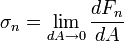
Fluid Mechanics for MAP/Differential Analysis of Fluid Flow
< Fluid Mechanics for MAP>back to Chapters of Fluid Mechanics for MAP
>back to Chapters of Microfluid Mechanics
Differential relations for a fluid particle
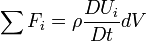
We are interested in the distribution of field properties at each point in space. Therefore, we analyze an infinitesimal region of a flow by applying the RTT to an infinitesimal control volume, or , to a infinitesimal fluid system.
Conservation of mass
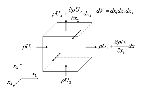
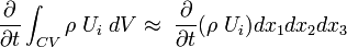
The conservation of mass according to RTT
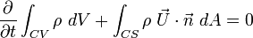
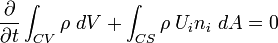
or in tensor form
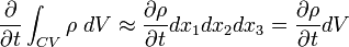
The differential volume is selected to be so small that density  can be accepted to be uniform within this volume. Thus the first integral in 1 is:
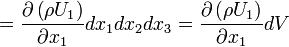
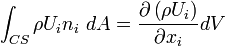
The flux term (second integral term) in the equation of conservation of mass can be analyzed in groups:

Let's look to the surfaces perpendicular to 
![\displaystyle
\int_{CS\, x_{1}}\rho U_i n_i\ dA = -\rho U_{1}dx_{2}dx_{3} + \left[\rho U_{1} + \frac{\partial\left(\rho U_{1}\right)}{\partial x_{1}}dx_{1}\right] dx_{2}dx_{3}](../I/m/b8daf676f847e686210f30a17b9082c2.png)
Similarly, the flux integrals through surfaces perpendicular to  and
and  are
are
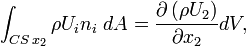
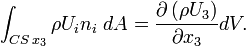
Hence the flux integral reads;
The conservation of mass equation becomes:
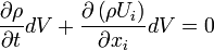
Droping the  , we reach to the final form of the conservation of mass:
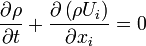
This equation is also called continuity equation. It can be written in vector form as:

For a steady flow, continuity equation becomes:

.
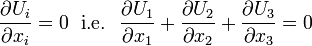
For incompresible flow, i.e.  :
:
Example
For a two dimensional, steady and incompressible flow in  plane given by:

Find how many possible  can exist.
For incompressible steady flow:

in two diemnsions
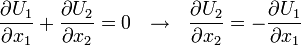
Thus,

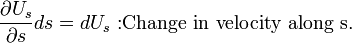
This is an expression for the rate of change of velocity while keeping
 constant. Therefore the integral of this equation reads
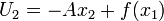
Thus, any function  is allowable.
Example
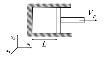
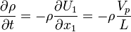
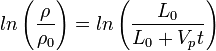
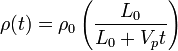
Consider one-dimensional flow in the piston. The piston suddenly moves with the velocity  . Assume uniform
  in the piston and a linear change of velocity
  such that
  at the bottom (
 ) and
) and  on the piston (
 ), i.e.

Obtain a function for the density as a function of time.
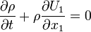
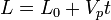
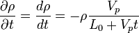
The conservation of mass equation is:
For one-dimensional flow and uniform  , this equaiton simplifies to
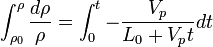
The same problem can be solved by using the integral approach with a deforming control volume.
The differential equation of linear momentum
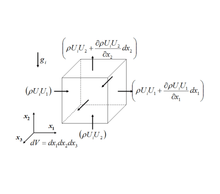
 (momentum per unit volume in i-direction) through the surfaces perpendicular to
  axis
axis
The integral equation for the momentum conservation is
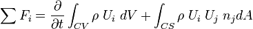
For the first integral we assume and  are uniform within dV, and dV is so small that:
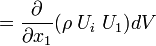
Analyze the flux of the  momentum terms through the faces perpendicular to the axis:

First consider the flux of (momentum per unit volume in i-direction) through the surfaces perpendicular to  axis:
axis:
![\displaystyle
\int_{CS\,x_{1}}\rho\;U_{i}\;U_{j}\;n_{j}\;dA = -\rho\;U_{i}\;U_{1}\;dx_{2}dx_{3}\; + \left[\rho\ U_{i}\ U_{1}\ dx_{2}\ dx_{3} + \frac{\partial}{\partial x_{1}}(\rho\ U_{i}\ U_{1})\ dx_{1}\right]dx_{2}\ dx_{3}](../I/m/19dfde29ec162d04407931e3a5a4a6ec.png)
Similarly, the momentum flux through the surfaces in other directions read
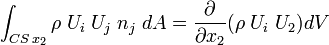
,
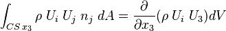
.
Rearranging the equation for  we obtain:
![\displaystyle \sum F_{i} = \left[\frac{\partial}{\partial t}(\rho\ U_{i}) + \frac{\partial}{\partial x_{j}}(\rho\ U_{i}\ U_{j})\right]dV](../I/m/22ebd3302d0618aaa547a8850d578cec.png)
We can simplify further:
![\displaystyle
\sum F_{i} = \left[U_{i}\frac{\partial \rho}{\partial t} + \rho\frac{\partial U_{i}}{\partial t} + U_{i} \frac{\partial}{\partial x_{j}}(\rho\;U_{j}) + \rho\;U_{j}\;\frac{\partial U_{i}}{\partial x_{j}}\right]dV](../I/m/ddcce0a44f887a28593533aed944b592.png)
![\displaystyle \sum F_{i}= U_{i}\underbrace{\left[\frac{\partial \rho}{\partial t}\;+ \frac{\partial}{\partial x_{j}}(\rho\;U_{j})\right]}_{continuity\ equation=0}dV\;+ \rho\underbrace{\left[\frac{\partial U_{i}}{\partial t}\;+ U_{j}\frac{\partial U_{i}}{\partial x_{j}}\right]}_{\frac{D U_{i}}{D t};subtantial\ derivative\ of\ U_i}dV](../I/m/1fee73b26730856f0f07814aa7312505.png)
Hence
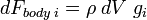
Let's look to the forces on the exposed on the diffrential control volume:
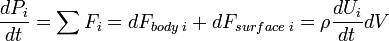
Here, only gravitational force is considered as a body force. Thus,
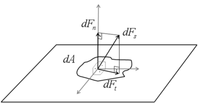
Surface forces are the stresses acting on the control surfaces.  can be resolved into three components.
  is normal to dA.
  are tangent to dA:
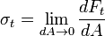
 is a normal stress whereas
  is a shear stress. The shear stresses are also designated by
  .
.
Thus, the surface forces are due to stresses on the surfaces of the control surface.
![\displaystyle
\sigma_{ij}=\left[
\begin{matrix}
\sigma_{11} & \sigma_{12} & \sigma_{13} \\
\sigma_{21} & \sigma_{22} & \sigma_{23} \\
\sigma_{31} & \sigma_{32} & \sigma_{33}
\end{matrix}
\right]](../I/m/7c88551fd5f0dcaaa0b23936319d4e32.png)
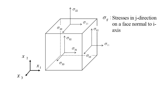
We define the positive direction for the stress as the positive coordinate direction on the surfaces (e.g. on ABCD) for which the outwards normal is in the positive coordinate direction . If the outward normal represents the negative direction (A'B'C'D'), then the stresses are considered positive if directed in the negative coordinate directions.
The stresses on the surface  are the sum of pressure plus the viscous stresses which arise from motion with velocity gradients:
![\displaystyle
\sigma_{ij}=\left[
\begin{matrix}
-P & 0 & 0 \\
0 & -P & 0 \\
0 & 0 & -P
\end{matrix}
\right]
+
\left[
\begin{matrix}
\tau_{11} & \tau_{12} & \tau_{13} \\
\tau_{21} & \tau_{22} & \tau_{23} \\
\tau_{31} & \tau_{32} & \tau_{33}
\end{matrix}
\right]=
\left[
\begin{matrix}
-P+\tau_{11} & \tau_{12} & \tau_{13} \\
\tau_{21} & -P+\tau_{22} & \tau_{23} \\
\tau_{31} & \tau_{32} & -P+\tau_{33}
\end{matrix}
\right]](../I/m/b5c866fed74b8df5f29f9e4a163ccfd2.png)
 has a minus sign since the force due to pressure acts opposite to the surface normal.
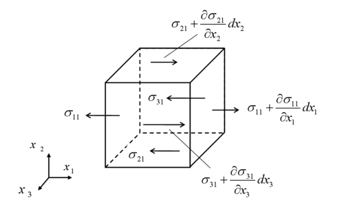
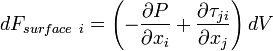
Let us look to the differential surface force in the direction:

Noting that 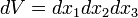 and
and  (4),
(4),
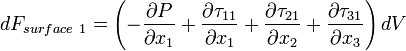
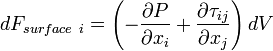
Thus in tensor form the differential surface forces in  'th direction can be written as
Note that  is a symmetric tensor, i.e.

Hence, the diffential surface forces reads:
Inserting  and
and  into (2),
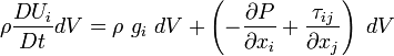
and canceling we obtain
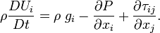
Expanding the substatial derivative at the left hand side,
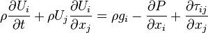
We obtain the the most general form of momentum equation which is valid for any fluid (Newtonian, Non-newtonian, Compressible, etc.). It is non-linear due to the  term at the LHS. Efect of Newtonian and Non-newtonian properties appears in the formulation of the viscous stresses . will introduce also non-linearity when the fluid is non-Newtonian.
It should be noted that these formulations are based on stress conception which was thought to exist in fluids in motion. However it is known that can be expressed as momentum transfer per unit area and time. Thus it can be considered as molecular momentum transport term. Derivations based on this concept requires a molecular approach (which is lengthy). The students should be aware that causes momentum transport when there is a gradient of velocity.
Linear momentum equation for Newtonian Fluid: "Navier-Stokes Equation"
For a Newtonian fluid, the viscous stresses are defined as:
![\displaystyle \tau_{ij} = \mu\left[\frac{\partial U_{i}}{\partial x_{j}} + \frac{\partial U_{j}}{\partial x_{i}}\right] - \frac{2}{3}\delta_{ij}\mu\frac{\partial U_{k}}{\partial x_{k}}](../I/m/9da430d12463eb77545a5bec4fe0cddc.png)
Note that derivation of this relation is beyond the scaope of this course.
Thus, the momentum equation (6) becomes
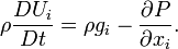
![\displaystyle \rho\frac{DU_{i}}{Dt} = \rho g_{i} - \frac{\partial P}{\partial x_{i}} + \frac{\partial}{\partial x_{j}}\left[\mu \left(\frac{\partial U_{i}}{\partial x_{j}} + \frac{\partial U_{j}}{\partial x_{i}}\right) - \frac{2}{3}\mu\ \delta_{ij}\ \frac{\partial U_{k}}{\partial x_{k}}\right]](../I/m/b016a98aa36ab2b8087d423325ae1d10.png)
For a flow with constant viscosity (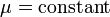 ):
):
![\displaystyle \rho\frac{DU_{i}}{Dt} = \rho g_{i} - \frac{\partial P}{\partial x_{i}} + \mu \frac{\partial}{\partial x_{j}}\left[\frac{\partial U_{i}}{\partial x_{j}} + \frac{\partial U_{j}}{\partial x_{i}} - \frac{2}{3}\delta_{ij}\ \frac{\partial U_{k}}{\partial x_{k}}\right]](../I/m/e2eae157717c5ced17516da9a64ade81.png)
since,
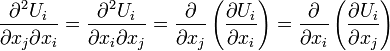
then,

For an incompressible flow
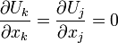
hence assuming that the viscosity is constant, it can be easily shown that the momentum equation reduces to

Euler's equation: Inviscid flow
When the velocity gradients in the flow is negligible and/or the Reynolds number takes very high values, the viscous stresses can be neglected:

Since, the viscous stresses are proportional to viscosity:

for flows, where is neglected, the flow is called frictionless or inviscid, although there is a finite viscosity of the flow. Accordingly, the linear momentum equation reduces to
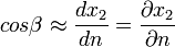
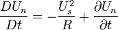
Euler's equation in streamline coordinates
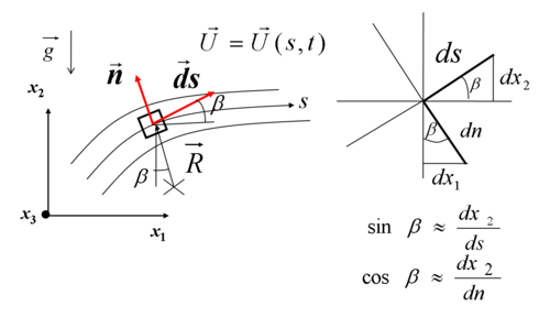
Euler's equation take a special form along and normal to a streamline with which one can see the dependency between the pressure, velocity and curvature of the streamline.
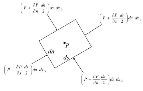
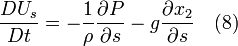
To obtain Euler's equation in s-direction, apply Newton's second law in s-direction in the absence of viscous forces.
![\displaystyle
\rho dV \left[\frac{\partial U_{s}}{\partial t} + U_{s}\frac{\partial U_{s}}{\partial s}\right]=
-\frac{\partial P}{\partial s}dV -\rho\ gsin\beta dV](../I/m/a62094420acd56cf0da7c90f8408949c.png)
Omitting would deliver
Since
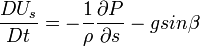
then the Equler's equation along a streamline reads
For a steady flow and by neglecting body forces,
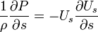
it can be seen that decrease in velocity means increase in pressure as is indicated by the Bernoulli equation.
To obtain Euler's equation in n direction, apply Newton's second law in the absence of viscous forces and for a steady flow.

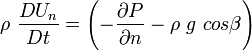
Since,
Then,
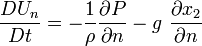
For a steady flow, the normal acceleration of the fluid is towards the center of curvature of the streamline:
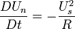
Hence,
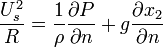
For an unsteady flow,
For steady flow neglecting body forces, the Euler's equation normal to the streamline is

which indicates that pressure increases in a direction outwards from the center of the curvature of the streamlines. In other words, pressure drops towards the center of curvature, which, consequently creates a potential difference in terms of pressure and forces the fluid to change its direction. For a straight streamline  , there is no pressure variation normal to the streamline.
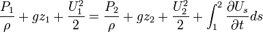
Bernoulli equation: Integration of Euler's equation along a streamline for a steady flow
For a steady flow, Euler's equation along a streamline reads,
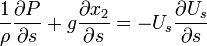
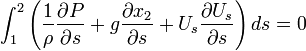
If a fluid particle moves a distance ds, along a streamline, since every variable becomes a function of  :
:
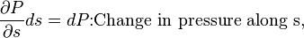
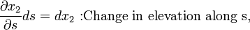
Integration of the Euler equation between two locations, 1 and 2, along reads
For incompressible flow  and after changing the notation as:
  and
and  , the integration results in
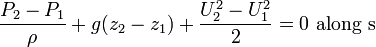
or in its most beloved form:
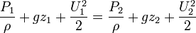
In other words along a streamline:
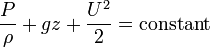
Note that due to the assumptions made during the derivation, the following restrictions applies to this equation: The flow should be steady, incompressible, frictionless and the equation is valid only along a streamline.
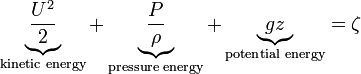
Different forms of Bernoulli equation
The common forms of Bernoulli equation are as follows:
Energy form (per unit mass)
Pressure form
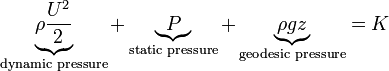
Head form
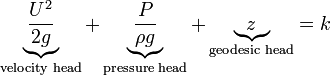
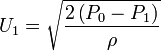
Static, stagnation and dynamic pressures
How do we measure pressure? When the streamlines are parallel to the wall we can use pressure taps.
|
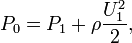
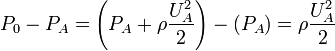
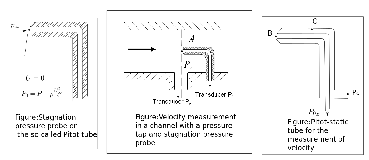
If the measured location is far from the wall, static pressure measurements can be made by a static pressure probe. The stagnation pressure is the value obtained when a flowing fluid is decelerated to zero velocity by a frictionless flow process. The Stagnation pressure can be calculated as follows: 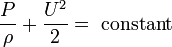 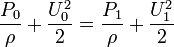
|
_Fernando_Alonso_pitot_probe.jpg) Pitot tube used in racing car |

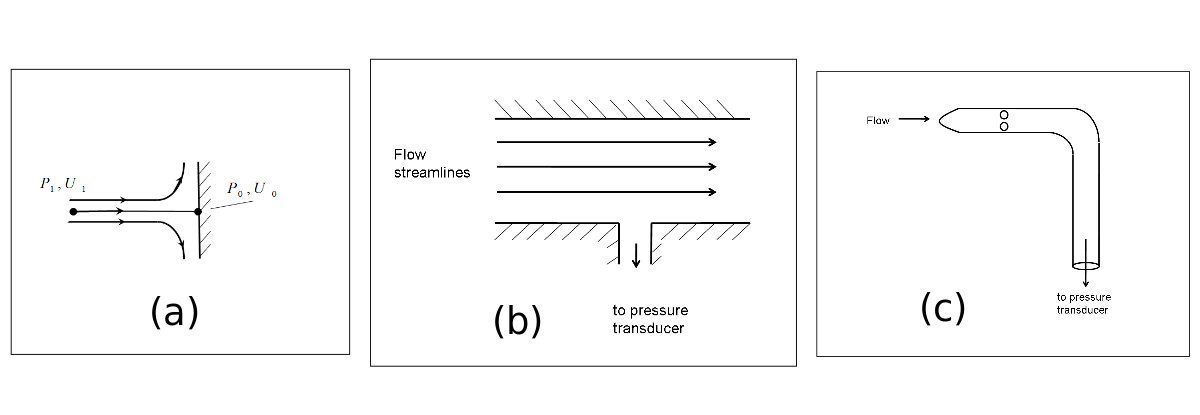
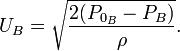
If we know the pressure difference  , we can calculate the
  velocity.
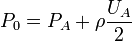
The stagnation pressure is measured in the laboratory using a probe that faces directly upstream flow.
Such a probe is called a stagnation pressure probe or Pitot tube . Thus, using a pressure tap and a Pitot tube one can measure local velocity:
Thus, measuring  one can determine
  .
.
|
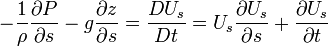
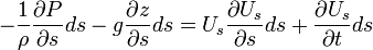
However, in the absence of a wall with well defined location, the velocity can be measured by a Pitot-static tube. The pressure is measured at B and C; assuming Hence,
|
 .
. 
Unsteady Bernoulli equation
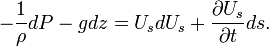
The Euler's equation along a streamline is:
along ds,
hence,
Integration between two points along a streamline is:
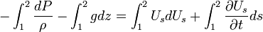
For incompressible flow, , thus the integral reads
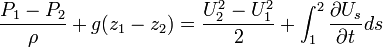
The unsetady Bernoulli equation involves the integration of the time gradient of the velocity between two points.: