Mathematics
Mathematics is about numbers (counting), quantity, and coordinates.
Notations
Notational locations Weight Oversymbol Exponent Coefficient Variable Operation Number Range Index
For each of the notational locations around the central Variable, conventions are often set by consensus as to use. For example, Exponent is often used as an exponent to a number or variable: 2-2 or x2.
A common Oversymbol is one for the average  .
.
Operation may be replaced by a function, for example.
All notational locations could look something like
bx 
x = n a 
f(x) n → ∞
where the center line means "a x Σ f(x)" for all added up values of f(x) when x = n from say 0 to infinity with each term in the sum before the summation is multiplied by bn, then divided by n for an average whenever n is finite.
Numbers


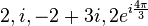
Natural numbers Integers Rational numbers Real numbers Complex numbers
"Scientific notation (more commonly known as standard form) is a way of writing numbers that are too big or too small to be conveniently written in decimal form. Scientific notation has a number of useful properties and is commonly used in calculators and by scientists, mathematicians and engineers."[1]
| Standard decimal notation | Normalized scientific notation |
|---|---|
| 2 | 2×100 |
| 300 | 3×10² |
| 4,321.768 | 4.321768×10³ |
| -53,000 | −5.3×10⁴ |
| 6,720,000,000 | 6.72×10⁹ |
| 0.2 | 2×10⁻¹ |
| 0.000 000 007 51 | 7.51×10⁻⁹ |
"A metric prefix or SI prefix is a unit prefix that precedes a basic unit of measure to indicate a decadic multiple or fraction of the unit. Each prefix has a unique symbol that is prepended to the unit symbol."[2]
| Metric prefixes | ||||||||||||||||||||||||||||||||||||||||||||||||||||||||||||||||||||||||||||||||||||||||||||||||||||||||||||||||||||||||||||||||||||||||||||||||||||||||||||||||||||||||||||||||||||||||
|---|---|---|---|---|---|---|---|---|---|---|---|---|---|---|---|---|---|---|---|---|---|---|---|---|---|---|---|---|---|---|---|---|---|---|---|---|---|---|---|---|---|---|---|---|---|---|---|---|---|---|---|---|---|---|---|---|---|---|---|---|---|---|---|---|---|---|---|---|---|---|---|---|---|---|---|---|---|---|---|---|---|---|---|---|---|---|---|---|---|---|---|---|---|---|---|---|---|---|---|---|---|---|---|---|---|---|---|---|---|---|---|---|---|---|---|---|---|---|---|---|---|---|---|---|---|---|---|---|---|---|---|---|---|---|---|---|---|---|---|---|---|---|---|---|---|---|---|---|---|---|---|---|---|---|---|---|---|---|---|---|---|---|---|---|---|---|---|---|---|---|---|---|---|---|---|---|---|---|---|---|---|---|---|---|
| ||||||||||||||||||||||||||||||||||||||||||||||||||||||||||||||||||||||||||||||||||||||||||||||||||||||||||||||||||||||||||||||||||||||||||||||||||||||||||||||||||||||||||||||||||||||||
"A significant figure is a digit in a number that adds to its precision. This includes all nonzero numbers, zeroes between significant digits, and zeroes indicated to be significant."[1]
"Leading and trailing zeroes are not significant because they exist only to show the scale of the number. Therefore, 1,230,400 has five significant figures—1, 2, 3, 0, and 4; the two zeroes serve only as placeholders and add no precision to the original number."[1]
"When a number is converted into normalized scientific notation, it is scaled down to a number between 1 and 10. All of the significant digits remain, but all of the place holding zeroes are incorporated into the exponent. Following these rules, 1,230,400 becomes 1.2304 x 10⁶."[1]
"It is customary in scientific measurements to record all the significant digits from the measurements"[1], for example, 1,230,400, but the measurement may have introduced an error which when calculated indcates the last significant digit has a range of values where the most likely one is the "4". The range may be 3-5 so that the last significant digit plus this error may be written as (4,1) meaning 4-1=3 and 4+1=5.
Another example of significant digists is the speed of all massless particles and associated fields—including electromagnetic radiation such as light—in vacuum ... [The most accurate value is] 299792.4562±0.0011 [km/s].[3]"[4] The magnitude of the speed is 299792.4562 and the actual measured variation is ±0.0011 so that the last two significant digits "62" are most likely within a variation from "51" to "73".
"Most calculators and many computer programs present very large and very small results in"[1] E notation. "[T]he letter E or e is often used to represent times ten raised to the power of (which would be written as "x 10b") [where b represents a number] and is followed by the value of the exponent."[1]
Def. "[a]ny real number that cannot be expressed as a ratio of two integers"[5] is called an irrational number.
Def. "[i]ncapable of being put into one-to-one correspondence with the natural numbers or any subset thereof"[6] is called uncountable.
An uncountable set of numbers such as the irrational numbers lies somewhere between a finite set of numbers, for example, the set of natural factors of 6: {1,2,3,6}, and an infinite set of numbers such as the natural numbers.
Def. "[t]he branch of pure mathematics concerned with the properties of integers"[7] is called number theory.
Theoretical mathematics
Def. "[a]n abstract representational system used in the study of numbers, shapes, structure and change and the relationships between these concepts"[8] is called mathematics.
Arithmetic
Notation: let the symbol > represent greater than.
For example, the integer five (5) is greater than the integer (2): 5 > 2.
Notation: let the symbol < represent less than also known as smaller than
For, example, 2 < 3.
Notation: let the relation symbol ≠ indicate that two expressions are different.
For example, 2 x 3 ≠ 5 x 7.
Notation: let the relation symbol ~ represent similar to.
For example, depending on the scale involved, 7 ~ 8 on a scale of 10, 7/10 = 0.7 and 8/10 = 0.8. relative to numbers between 0.5 and 1.0, 0.7 ~ 0.8, but 0.2 ≁ 0.7.
Similarity may be close such as 0.7 ≈ 0.8, but 0.5 ~ 0.8. Or similarity may include equality, 5 ± 3 ≃ 4 ± 2. When the degree of equality is greater than the degree of similarity, the symbol ≅ is used. The reverse is represented by ≊.
Def. "[t]he mathematics of numbers (integers, rational numbers, real numbers, or complex numbers) under the operations of addition, subtraction, multiplication, and division"[9] is called an arithmetic.
Def. "[a] symbol ( = ) used in mathematics to indicate that two values are the same"[10]
Consider the integers: 1 and 2. The statement, "1 + 2 = 3", contains the operation + (addition) and the relation = (equals).
The exponent can require a different operator of arithmetic.
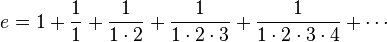
"The number  is an important mathematical constant, approximately equal to 2.71828, that is the base of the natural logarithm.[11]"[12]
- e2 + e3 ≠ e5. Yet
- e2 x e3 = e(2 + 3) = e5.
Usually, pure arithmetic only involves numbers. But, when arithmetic is used in a science such as radiation astronomy, dimensional analysis is also applicable.
To build an observatory usually requires adding components together.
- 1 dome + 1 telescope + 1 outbuilding + 1 control room + 1 laboratory + 1 observation room may = 1 observatory.
Yet,
- 1 + 1 + 1 + 1 + 1 + 1 = 6 components in 1 simple observatory.
However, attempting to add 1 dome to 1 telescope may have little or no meaning. The operation of addition would be similar to the operation of construction.
If 1 G2V star is added to 1 M2V star the result may be a double star. The operation of addition here usually requires an explanation (a theory).
Algebra
Notation: let the symbol * designate an as yet unspecified operation.
Notation: let the symbol R designate an as yet unspecified relation.
Def. "[a] system for computation using letters or other symbols to represent numbers, with rules for manipulating these symbols"[13] is called an algebra.
Fundamentally, algebra uses letters to represent as yet unspecified numbers. The numbers may be integers, rational numbers, irrational numbers, or any real number or complex number. As an experimentalist, eventually you must find a way to change unspecified numbers into specified ones. But, as a theoretician, first you are free to leave the numbers in some algebraic form, then to have your theory tested by any experimentalist you need to relate the algebraic terms of your theory to real or complex numbers.
Consider the lower case letters of the English alphabet: a and n. The statement, "a * n R an", contains the operation * (followed by) and the relation R (spells the word).
The manipulations of these symbols are performed using operations.
Def. "a procedure for generating a value from one or more other values (the operands; the value for any particular [operand] is unique)"[14] is called an operation.
Notation: let the symbol represent the summation of many terms.
Notation: let the symbol  represent the product of many terms.
The results are recorded using statements of relation.
Def. "[a] relation in which each element of the domain is associated with exactly one element of the codomain"[15] is called a function.
Geometry

Def. "[o]f geometrical figures including triangles, squares, ellipses, arcs and more complex figures, having the same shape but possibly different size, rotational orientation, and position; in particular, having corresponding angles equal and corresponding line segments proportional; such that one can be had from the other using a sequence of operations of rotation, translation and scaling"[16] is called similar.
Def. "a branch of mathematics that studies solutions of systems of algebraic equations using both algebra and geometry"[17] is called algebraic geometry.
Def. "a branch of mathematics that investigates properties of figures through the coordinates of their points"[18] is called analytic geometry.
Def. "a branch of mathematics that investigates those properties of figures that are invariant when projected from a point to a line or plane"[19] is called projective geometry.
The universe as often perceived may be described spatially, sometimes with plane geometry, other occasions with spherical geometry.
Def. "[t]he act of turning around a centre or an axis"[20] is called a rotation.
"A rotation is a circular movement of an object around a center (or point) of rotation. A three-dimensional object rotates always around an imaginary line called a rotation axis. If the axis is within the body, and passes through its center of mass the body is said to rotate upon itself, or spin. A rotation about an external point, e.g. the Earth about the Sun, is called a revolution or orbital revolution"[21]
Def. "the traversal of one body through an orbit around another body"[22] is called a revolution.
Conic sections
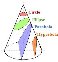
Def. "[a]ny of the four distinct shapes that are the intersections of a cone with a plane, namely the circle, ellipse, parabola and hyperbola"[23] is called a conic section.
"In mathematics, a conic section (or just conic) is a curve obtained as the intersection of a cone (more precisely, a right circular conical surface) with a plane."[24]
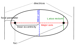
"Various parameters are associated with a conic section, as shown in the following table. (For the ellipse, the table gives the case of a>b, for which the major axis is horizontal; for the reverse case, interchange the symbols a and b. For the hyperbola the east-west opening case is given. In all cases, a and b are positive.)"[24].
| conic section | equation | eccentricity (e) | linear eccentricity (c) | semi-latus rectum (ℓ) | focal parameter (p) |
|---|---|---|---|---|---|
| circle |  |
 |
|
 |
 |
| ellipse | 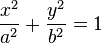 |
 |
 |
 |
 |
| parabola |  |
 |
|
 |
|
| hyperbola | 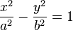 |
 |
 |
|
 |
Spherical geometry
.jpg)
Def. "[t]he non-Euclidean geometry on the surface of a sphere"[25] is called spherical geometry.
"Spherical geometry is the geometry of the two-dimensional surface of a sphere. It is an example of a geometry which is not Euclidean. Two practical applications of the principles of spherical geometry are to navigation and astronomy."[26]
"A sphere [suggested by the image of the Earth at right] is not a Euclidean space, but locally the laws of the Euclidean geometry are good approximations. In a small triangle on the face of the earth, the sum of the angles is very nearly 180. The surface of a sphere can be represented by a collection of two dimensional maps. Therefore it is a two dimensional manifold."[26]
"The great-circle or [Great Circle] orthodromic distance is the shortest distance between any two points on the surface of a sphere measured along a path on the surface of the sphere (as opposed to going through the sphere's interior). Because spherical geometry is different from ordinary Euclidean geometry, the equations for distance take on a different form. The distance between two points in Euclidean space is the length of a straight line from one point to the other. On the sphere, however, there are no straight lines. In non-Euclidean geometry, straight lines are replaced with geodesics. Geodesics on the sphere are the great circles (circles on the sphere whose centers are coincident with the center of the sphere)."[27]
"Through any two points on a sphere which are not directly opposite each other, there is a unique great circle. The two points separate the great circle into two arcs. The length of the shorter arc is the great-circle distance between the points. A great circle endowed with such a distance is the Riemannian circle."[27]
Trigonometry
Def. "the relationships between the sides and the angles of triangles and the calculations based on them"[28] is called trigonometry.
"Trigonometry ... studies triangles and the relationships between their sides and the angles between these sides. Trigonometry defines the trigonometric functions, which describe those relationships and have applicability to cyclical phenomena, such as waves."[29]
Calculus
Notation: let the symbol  represent change in.
Notation: let the symbol  represent an infinitesimal change in.
Notation: let the symbol  represent an infinitesimal change in one of more than one.
Let

be a function where values of  may be any real number and values resulting in
  are also any real number.
-
 is a small finite change in which when put into the function
  produces a
  .
.
These small changes can be manipulated with the operations of arithmetic: addition ( ), subtraction (), multiplication (
 ), and division (
 ).
).

Dividing by and taking the limit as → 0, produces the slope of a line tangent to f(x) at the point x.
For example,


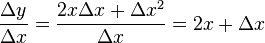
as and go towards zero,

This ratio is called the derivative.
Let

then


where z is held constant and

where x is held contstant.
Notation: let the symbol  be the gradient, i.e., derivatives for multivariable functions.

For
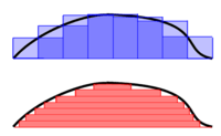
![\Delta x * \Delta y = [f(x + \Delta x) - f(x)] * \Delta x](../I/m/6da4993c799821d9a1d81ba4727956af.png)
the area under the curve shown in the diagram at right is the light purple rectangle plus the dark purple rectangle in the top figure

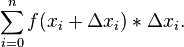
Any particular individual rectangle for a sum of rectangular areas is

The approximate area under the curve is the sum of all the individual (i) areas from i = 0 to as many as the area needed (n):
Notation: let the symbol  represent the integral.
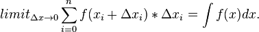
This can be within a finite interval [a,b]

when i = 0 the integral is evaluated at  and i = n the integral is evaluated at
  . Or, an indefinite integral (without notation on the integral symbol) as n goes to infinity and i = 0 is the integral evaluated at x = 0.
Def. a branch of mathematics that deals with the finding and properties ... of infinitesimal differences [or changes] is called a calculus.
"Calculus [focuses] on limits, functions, derivatives, integrals, and infinite series."[30]
"Although calculus (in the sense of analysis) is usually synonymous with infinitesimal calculus, not all historical formulations have relied on infinitesimals (infinitely small numbers that are nevertheless not zero)."[31]
Line integrals
Def. an "integral the domain of whose integrand is a curve"[32] is called a line integral.
"The pulsar dispersion measures [(DM)] provide directly the value of

along the line of sight to the pulsar, while the interstellar Hα intensity (at high Galactic latitudes where optical extinction is minimal) is proportional to the emission measure"[33]
Vectors
Def. a "directed quantity, one with both magnitude and direction; the signed difference between two points"[34] is called a vector.
"An observed time series consists of N data values x(tα) taken at a set of N discrete times {tα}. Hence it defines an N-dimensional contravariant vector in sampling space, by taking as the αth component of the vector, the value of the data at time tα, i.e.,
![x^\alpha = [x({t_1}),x({t_2}),...,x({t_N})].](../I/m/4db34b0253f10db9d6330a6da256b55f.png)
This representation is the canonical basis for sampling space."[35]
Tensors
Def. a "mathematical object consisting of a set of components with n indices each of which range from 1 to m where n is the rank and m is the dimension"[36] is called a tensor.
"An impressive array of time series analysis methods are equivalent to treating the data as a vector in function space, then projecting the data vector onto a subspace of low dimension. A geometric approach isolates and exposes many of the important features of time series techniques, directly adapts to irregular time spacing, and easily accommodates variable statistical weights. Tensor notation provides an ideal formalism for these techniques. It is quite convenient for distinguishing a variety of different vector spaces, and is the most compact notation for all the sums which arise in the analysis."[35]
"[T]he generally invariant line element

[contains] the spacetime metric tensor  [which] plays a dual role: on the one hand it determines the spacetime geometry, on the other it represents the (ten components of the) gravitational potential, and is thus a dynamical variable."[37]
Electronic computers
Def. "[a] programmable electronic device that performs mathematical calculations and logical operations, especially one that can process, store and retrieve large amounts of data very quickly; now especially, a small one for personal or home use employed for manipulating text or graphics, accessing the Internet, or playing games or media"[38] is called a computer.
"A computer is a general purpose device that can be programmed to carry out a finite set of arithmetic or logical operations. Since a sequence of operations can be readily changed, the computer can solve more than one kind of problem."[39]
Programming
"A computer program (also software, or just a program) is a sequence of instructions written to perform a specified task with a computer.[40] A computer requires programs to function, typically executing the program's instructions in a central processor.[41]"[42]
"Computer programming (often shortened to programming or coding) is the process of designing, writing, testing, debugging, and maintaining the source code of computer programs."[43]
Probability
Def. "a number, between 0 and 1, expressing the precise likelihood of an event happening"[44] is called a probability.
"Probability is a measure of the expectation that an event will occur or a statement is true. Probabilities are given a value between 0 (will not occur) and 1 (will occur).[45] The higher the probability of an event, the more certain we are that the event will occur."[46]
Statistics
Def. "[a] mathematical science concerned with data collection, presentation, analysis, and interpretation"[47] is called statistics.
"Statistics is the study of the collection, organization, analysis, interpretation, and presentation of data.[48][49] It deals with all aspects of this, including the planning of data collection in terms of the design of surveys and experiments.[48]"[50]
Research
Hypothesis:
- Mathematics can be described with set theory.
Control groups

The findings demonstrate a statistically systematic change from the status quo or the control group.
“In the design of experiments, treatments [or special properties or characteristics] are applied to [or observed in] experimental units in the treatment group(s).[51] In comparative experiments, members of the complementary group, the control group, receive either no treatment or a standard treatment.[52]"[53]
Proof of concept
Def. a “short and/or incomplete realization of a certain method or idea to demonstrate its feasibility"[54] is called a proof of concept.
Def. evidence that demonstrates that a concept is possible is called proof of concept.
The proof-of-concept structure consists of
- background,
- procedures,
- findings, and
- interpretation.[55]
See also
- Portal:Mathematics
References
- 1 2 3 4 5 6 7 "Scientific notation, In: Wikipedia". San Francisco, California: Wikimedia Foundation, Inc. January 25, 2013. Retrieved 2013-01-30.
- ↑ "Metric prefix, In: Wikipedia". San Francisco, California: Wikimedia Foundation, Inc. January 21, 2013. Retrieved 2013-02-01.
- ↑ Evenson, KM; et al. (1972). "Speed of Light from Direct Frequency and Wavelength Measurements of the Methane-Stabilized Laser". Physical Review Letters 29 (19): 1346–49. doi:10.1103/PhysRevLett.29.1346.
- ↑ "Speed of light, In: Wikipedia". San Francisco, California: Wikimedia Foundation, Inc. December 10, 2012. Retrieved 2012-12-24.
- ↑ "irrational number, In: Wiktionary". San Francisco, California: Wikimedia Foundation, Inc. November 10, 2012. Retrieved 2013-02-01.
- ↑ "uncountable, In: Wiktionary". San Francisco, California: Wikimedia Foundation, Inc. October 16, 2012. Retrieved 2013-02-01.
- ↑ "number theory, In: Wiktionary". San Francisco, California: Wikimedia Foundation, Inc. November 10, 2012. Retrieved 2013-02-01.
- ↑ "mathematics, In: Wiktionary". San Francisco, California: Wikimedia Foundation, Inc. January 13, 2013. Retrieved 2013-01-31.
- ↑ "arithmetic, In: Wiktionary". San Francisco, California: Wikimedia Foundation, Inc. January 13, 2013. Retrieved 2013-01-31.
- ↑ "equal sign, In: Wiktionary". San Francisco, California: Wikimedia Foundation, Inc. December 13, 2012. Retrieved 2013-01-31.
- ↑ Oxford English Dictionary, 2nd ed.: natural logarithm
- ↑ "e (mathematical constant), In: Wikipedia". San Francisco, California: Wikimedia Foundation, Inc. January 20, 2013. Retrieved 2013-02-01.
- ↑ "algebra, In: Wiktionary". San Francisco, California: Wikimedia Foundation, Inc. December 30, 2012. Retrieved 2013-01-31.
- ↑ "operation, In: Wiktionary". San Francisco, California: Wikimedia Foundation, Inc. December 22, 2012. Retrieved 2013-01-31.
- ↑ "function, In: Wiktionary". San Francisco, California: Wikimedia Foundation, Inc. January 16, 2013. Retrieved 2013-02-01.
- ↑ "similar, In: Wiktionary". San Francisco, California: Wikimedia Foundation, Inc. January 13, 2013. Retrieved 2013-01-31.
- ↑ "algebraic geometry, In: Wiktionary". San Francisco, California: Wikimedia Foundation, Inc. November 9, 2012. Retrieved 2013-01-31.
- ↑ "analytic geometry, In: Wiktionary". San Francisco, California: Wikimedia Foundation, Inc. November 9, 2012. Retrieved 2013-01-31.
- ↑ "projective geometry, In: Wiktionary". San Francisco, California: Wikimedia Foundation, Inc. October 17, 2012. Retrieved 2013-01-31.
- ↑ "rotation, In: Wiktionary". San Francisco, California: Wikimedia Foundation, Inc. January 11, 2013. Retrieved 2013-02-01.
- ↑ "Rotation, In: Wikipedia". San Francisco, California: Wikimedia Foundation, Inc. January 18, 2013. Retrieved 2013-02-01.
- ↑ "revolution, In: Wiktionary". San Francisco, California: Wikimedia Foundation, Inc. January 13, 2013. Retrieved 2013-02-01.
- ↑ "conic section, In: Wiktionary". San Francisco, California: Wikimedia Foundation, Inc. January 15, 2013. Retrieved 2013-01-31.
- 1 2 "Conic section, In: Wikipedia". San Francisco, California: Wikimedia Foundation, Inc. January 20, 2013. Retrieved 2013-01-31.
- ↑ "spherical geometry, In: Wiktionary". San Francisco, California: Wikimedia Foundation, Inc. 01 February 2013. Retrieved 2013-02-01.
- 1 2 "Spherical geometry, In: Wikipedia". San Francisco, California: Wikimedia Foundation, Inc. December 29, 2012. Retrieved 2013-02-01.
- 1 2 "Great-circle distance, In: Wikipedia". San Francisco, California: Wikimedia Foundation, Inc. January 22, 2013. Retrieved 2013-02-01.
- ↑ "trigonometry, In: Wiktionary". San Francisco, California: Wikimedia Foundation, Inc. October 16, 2012. Retrieved 2013-01-31.
- ↑ "Trigonometry, In: Wikipedia". San Francisco, California: Wikimedia Foundation, Inc. October 12, 2012. Retrieved 2012-10-14.
- ↑ "Calculus, In: Wikipedia". San Francisco, California: Wikimedia Foundation, Inc. October 13, 2012. Retrieved 2012-10-14.
- ↑ "infinitesimal calculus, In: Wiktionary". San Francisco, California: Wikimedia Foundation, Inc. Setember 19, 2012. Retrieved 2013-01-31.
- ↑ "line integral, In: Wiktionary". San Francisco, California: Wikimedia Foundation, Inc. September 18, 2013. Retrieved 2013-12-17.
- ↑ R. J. Reynolds (May 1, 1991).
 . The Astrophysical Journal 372 (05): L17-20. doi:10.1086/186013. http://adsabs.harvard.edu/full/1991ApJ...372L..17R. Retrieved 2013-12-17.
 - ↑ "title, In: Wiktionary". San Francisco, California: Wikimedia Foundation, Inc. December 10, 2013. Retrieved 2013-12-16.
- 1 2 Grant Foster (January 1996). "Time Series Analysis by Projection. II. Tensor Methods for Time Series Analysis". The Astronomical Journal 111 (1): 555-65. http://adsabs.harvard.edu/full/1996AJ....111..555F. Retrieved 2013-12-16.
- ↑ "title, In: Wiktionary". San Francisco, California: Wikimedia Foundation, Inc. November 20, 2013. Retrieved 2013-12-16.
- ↑ Jiří Bičák (2000). "Selected Solutions of Einstein's Field Equations: Their Role in General Relativity and Astrophysics, In: Einstein’s Field Equations and Their Physical Implications". Lecture Notes in Physics (Berlin: Springer Berlin Heidelberg) 540: 1-126. doi:10.1007/3-540-46580-4_1. ISBN 978-3-540-67073-5. http://arxiv.org/pdf/gr-qc/0004016. Retrieved 2013-07-04.
- ↑ "computer". Wiktionary (San Francisco, California: Wikimedia Foundation, Inc). January 31, 2013. http://en.wiktionary.org/wiki/computer. Retrieved 2013-01-31.
- ↑ "Computer, In: Wikipedia". San Francisco, California: Wikimedia Foundation, Inc. October 6, 2012. Retrieved 2012-10-14.
- ↑ Stair, Ralph M., et al. (2003). Principles of Information Systems, Sixth Edition. Thomson Learning, Inc.. pp. 132. ISBN 0-619-06489-7.
- ↑ Silberschatz, Abraham (1994). Operating System Concepts, Fourth Edition. Addison-Wesley. pp. 58. ISBN 0-201-50480-4.
- ↑ "Computer program". Wikipedia (San Francisco, California: Wikimedia Foundation, Inc). October 3, 2012. http://en.wikipedia.org/wiki/Computer_program. Retrieved 2012-10-14.
- ↑ "Computer programming, In: Wikipedia". San Francisco, California: Wikimedia Foundation, Inc. October 12, 2012. Retrieved 2012-10-14.
- ↑ "probability, In: Wiktionary". San Francisco, California: Wikimedia Foundation, Inc. January 13, 2013. Retrieved 2013-01-31.
- ↑ William Feller (June 2012). An Introduction to Probability Theory and its Applications. 1). ISBN 0-471-25708-7.
- ↑ "Probability, In: Wikipedia". San Francisco, California: Wikimedia Foundation, Inc. October 2, 2012. Retrieved 2012-10-14.
- ↑ "statistics, In: Wiktionary". San Francisco, California: Wikimedia Foundation, Inc. January 13, 2013. Retrieved 2013-01-31.
- 1 2 Dodge, Y. (2003) The Oxford Dictionary of Statistical Terms, OUP. ISBN 0-19-920613-9
- ↑ The Free Online Dictionary
- ↑ "Statistics, In: Wikipedia". San Francisco, California: Wikimedia Foundation, Inc. October 12, 2012. Retrieved 2012-10-14.
- ↑ Klaus Hinkelmann, Oscar Kempthorne (2008). Design and Analysis of Experiments, Volume I: Introduction to Experimental Design (2nd ed.). Wiley. ISBN 978-0-471-72756-9. http://books.google.com/?id=T3wWj2kVYZgC&printsec=frontcover.
- ↑ R. A. Bailey (2008). Design of comparative experiments. Cambridge University Press. ISBN 978-0-521-68357-9. http://www.cambridge.org/uk/catalogue/catalogue.asp?isbn=9780521683579.
- ↑ "Treatment and control groups, In: Wikipedia". San Francisco, California: Wikimedia Foundation, Inc. May 18, 2012. Retrieved 2012-05-31.
- ↑ "proof of concept, In: Wiktionary". San Francisco, California: Wikimedia Foundation, Inc. November 10, 2012. Retrieved 2013-01-13.
- ↑ Ginger Lehrman and Ian B Hogue, Sarah Palmer, Cheryl Jennings, Celsa A Spina, Ann Wiegand, Alan L Landay, Robert W Coombs, Douglas D Richman, John W Mellors, John M Coffin, Ronald J Bosch, David M Margolis (August 13, 2005). "Depletion of latent HIV-1 infection in vivo: a proof-of-concept study". Lancet 366 (9485): 549-55. doi:10.1016/S0140-6736(05)67098-5. http://www.ncbi.nlm.nih.gov/pmc/articles/PMC1894952/. Retrieved 2012-05-09.
External links
- Maths Problem Solving
- African Journals Online
- Bing Advanced search
- Google Books
- Google scholar Advanced Scholar Search
- International Astronomical Union
- JSTOR
- Lycos search
- NASA's National Space Science Data Center
- NCBI All Databases Search
- Office of Scientific & Technical Information
- Questia - The Online Library of Books and Journals
- SAGE journals online
- The SAO/NASA Astrophysics Data System
- Scirus for scientific information only advanced search
- SDSS Quick Look tool: SkyServer
- SIMBAD Astronomical Database
- SIMBAD Web interface, Harvard alternate
- Spacecraft Query at NASA.
- SpringerLink
- Taylor & Francis Online
- Universal coordinate converter
- Wiley Online Library Advanced Search
- Yahoo Advanced Web Search
| ||||||||||||||||||||||||||||||||||||||||||||
![]() This is a research project at http://en.wikiversity.org
This is a research project at http://en.wikiversity.org
| |
Development status: this resource is experimental in nature. |
| |
Educational level: this is a research resource. |
| |
Resource type: this resource is an article. |
| |
Resource type: this resource contains a lecture or lecture notes. |
| |
Subject classification: this is a mathematics resource . |