MacLaurin series
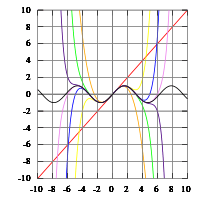
A MacLaurin series is a Taylor series that has a term at (0,0).
Calculus
Notation: let the symbol  represent change in.
Notation: let the symbol  represent an infinitesimal change in.
Notation: let the symbol  represent an infinitesimal change in one of more than one.
Let

be a function where values of  may be any real number and values resulting in
  are also any real number.
-
 is a small finite change in which when put into the function
  produces a
  .
.
These small changes can be manipulated with the operations of arithmetic: addition ( ), subtraction (
 ), multiplication (
 ), and division (
 ).
).

Dividing by and taking the limit as → 0, produces the slope of a line tangent to f(x) at the point x.
For example,


as and go towards zero,

This ratio is called the derivative.
Let

then


where z is held constant and

where x is held contstant.
Notation: let the symbol  be the gradient, i.e., derivatives for multivariable functions.

For
![\Delta x * \Delta y = [f(x + \Delta x) - f(x)] * \Delta x](../I/m/6da4993c799821d9a1d81ba4727956af.png)
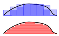
the area under the curve shown in the diagram at right is the light purple rectangle plus the dark purple rectangle in the top figure

Any particular individual rectangle for a sum of rectangular areas is

The approximate area under the curve is the sum  of all the individual (i) areas from i = 0 to as many as the area needed (n):

Notation: let the symbol  represent the integral.
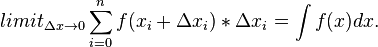
This can be within a finite interval [a,b]

when i = 0 the integral is evaluated at  and i = n the integral is evaluated at
  . Or, an indefinite integral (without notation on the integral symbol) as n goes to infinity and i = 0 is the integral evaluated at x = 0.
Def. a branch of mathematics that deals with the finding and properties ... of infinitesimal differences [or changes] is called a calculus.
"Calculus [focuses] on limits]], functions, derivatives, integrals, and infinite series."[1]
"Although calculus (in the sense of analysis) is usually synonymous with infinitesimal calculus, not all historical formulations have relied on infinitesimals (infinitely small numbers that are nevertheless not zero)."[2]
Series
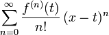
Taylor Series:

where fn refers to the number (n) of derivatives taken.
A MacLaurin series of a function ƒ(x) for which a derivative may be taken of the function or any of its derivatives at 0 is the power series

which can be written in the more compact sigma, or summation, notation as
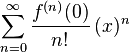
where n! denotes the factorial of n and ƒ (n)(0) denotes the nth derivative of ƒ evaluated at the point 0. The derivative of order zero ƒ is defined to be ƒ itself and (x)0 and 0! are both defined to be 1.
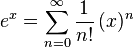
MacLaurin series for ex
Taylor series is defined as

The MacLaurin series occurs when t=0
The derivatives are


.
.
.
Development of MacLaurin series for 
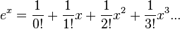
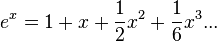
Explicit form can be written as
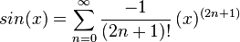
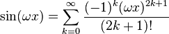
MacLaurin series for sin(x)


.
.
.
Development of MacLaurin series for 

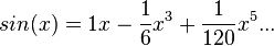
Explicit form can be written as
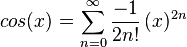
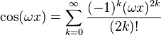
MacLaurin series for cos(x)
Development of MacLaurin series for 


.
.
.
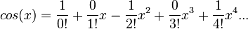
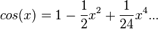
Explicit form can be written as
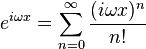
Euler's formula
Recalling Euler's Formula:

Recall the Taylor Series from above for at : (also called the MacLaurin series)

By replacing x with  , the Taylor series for
  can be found:
even powers of n = 2k:

odd powers of n = 2k+1:

For :
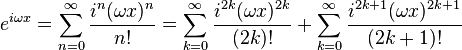
Using the two previous equations:
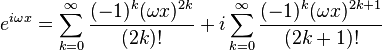

Therefore, the first part of the equation is equal to the Taylor series for cosine, and the second part is equal to the Taylor series for sine as follows:
MacLaurin series for 

| | |
 |  |
 |  |
 |  |
 |  |
| And so on.. | .. |
Rewriting the Maclaurin series expansion,

Substituting the values from the table, we get

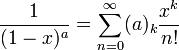
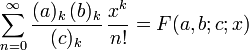
Using


We can represent

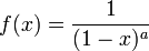
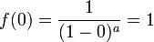
MacLaurin series for 
We have the function
Expand
| | |
 | 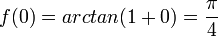 |
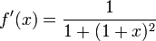 | 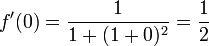 |
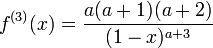
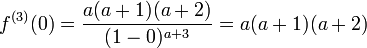
![f' '(x) = \frac {-2(x+1)}{\left[1+(1+x)^2\right]^2}](../I/m/c4dec210d8f453825158713858652d07.png) | ![f' '(0) = \frac {-2(0+1)}{\left[1+(1+0)^2\right]^2}= \frac{-1}{2}](../I/m/9dba7c973cf7b5b4f34a9cc2f37d809b.png) |
![f^{(3)}(x) = \frac {2(3x^2+6x+2)}{\left[1+(1+x)^2\right]^3}](../I/m/d07d44afc40c511874cad803795aa2f5.png) | ![f^{(3)}(0) = \frac {2(3(0)^2+6(0)+2)}{\left[1+(1+0)^2\right]^3} = \frac{1}{2}](../I/m/2b527a8a5cc698cf00da3076ebf07f87.png) |
| And so on.. | .. |
Rewriting the Maclaurin series expansion,

Substituting the values from the table, we get

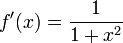
MacLaurin series for 
Expanding using Maclaurin's series
| | |
 |  |
 |  |
![f' '(x) = \frac {-2x}{\left[1+(x)^2\right]^2}](../I/m/a87d929c7391f12195f9a1b2219cf1b0.png) | ![f' '(0) = \frac {-2(0)}{\left[1+(0)^2\right]^2}= 0](../I/m/6b025f5cca00da3b14602f8ca6598b09.png) |
![f^{(3)}(x) = \frac {6x^2-2}{\left[1+(x)^2\right]^3}](../I/m/63da733e93098ceb0dcc0f285df6f1bc.png) | ![f^{(3)}(0) = \frac {6(0)^2-2)}{\left[1+(0)^2\right]^3} = -2](../I/m/0c25adfbbdfebadce1359850608b5b84.png) |
![f^{(4)}(x) = \frac {-24x(x^2-1}{\left[1+(x)^2\right]^4}](../I/m/82beb91be4b6b14b1b670e51712e29ba.png) | ![f^{(4)}(0) = \frac {-24(0)((0)^2-1}{\left[1+(0)^2\right]^4}= 0](../I/m/4570dc9a4f1f135eb1192b954a8b6304.png) |
![f^{(5)}(x) = \frac {24(5x^4-10x^2+1}{\left[1+(x)^2\right]^5}](../I/m/1e9579d4154ae3290c02706371375987.png) | ![f^{(5)}(x) = \frac {24(5(0)^4-10(0)^2+1}{\left[1+(0)^2\right]^5} = 24](../I/m/79ecd310e75ca8612a08ad57ea401b1a.png) |
| And so on.. | .. |
Rewriting the Maclaurin series expansion,

Substituting the values from the table, we get

Engineering
The "performance of a Markov system under different operating strategies [can be estimated] by observing the behavior of the system under the [strategy of having] a Maclaurin series for the performance measures of [the] Markov chains."[3]
Research
Hypothesis:
- Any non-convergent function can be represented by a MacLaurin series.
Control groups

The findings demonstrate a statistically systematic change from the status quo or the control group.
“In the design of experiments, treatments [or special properties or characteristics] are applied to [or observed in] experimental units in the treatment group(s).[4] In comparative experiments, members of the complementary group, the control group, receive either no treatment or a standard treatment.[5]"[6]
Proof of concept
Def. a “short and/or incomplete realization of a certain method or idea to demonstrate its feasibility"[7] is called a proof of concept.
Def. evidence that demonstrates that a concept is possible is called proof of concept.
The proof-of-concept structure consists of
- background,
- procedures,
- findings, and
- interpretation.[8]
See also
- Solution for sin(t)
- Solutions to problem set 2.7
References
- ↑ "Calculus, In: Wikipedia". San Francisco, California: Wikimedia Foundation, Inc. October 13, 2012. Retrieved 2012-10-14.
- ↑ "infinitesimal calculus, In: Wiktionary". San Francisco, California: Wikimedia Foundation, Inc. Setember 19, 2012. Retrieved 2013-01-31.
- ↑ Xi-Ren Cao (1998). "The Maclaurin Series for Performance Functions of Markov Chains". Advances in Applied Probability 30: 676-92. http://www.ece.ust.hk/~eecao/paper/60.pdf. Retrieved 2014-07-23.
- ↑ Klaus Hinkelmann, Oscar Kempthorne (2008). Design and Analysis of Experiments, Volume I: Introduction to Experimental Design (2nd ed.). Wiley. ISBN 978-0-471-72756-9. http://books.google.com/?id=T3wWj2kVYZgC&printsec=frontcover.
- ↑ R. A. Bailey (2008). Design of comparative experiments. Cambridge University Press. ISBN 978-0-521-68357-9. http://www.cambridge.org/uk/catalogue/catalogue.asp?isbn=9780521683579.
- ↑ "Treatment and control groups, In: Wikipedia". San Francisco, California: Wikimedia Foundation, Inc. May 18, 2012. Retrieved 2012-05-31.
- ↑ "proof of concept, In: Wiktionary". San Francisco, California: Wikimedia Foundation, Inc. November 10, 2012. Retrieved 2013-01-13.
- ↑ Ginger Lehrman and Ian B Hogue, Sarah Palmer, Cheryl Jennings, Celsa A Spina, Ann Wiegand, Alan L Landay, Robert W Coombs, Douglas D Richman, John W Mellors, John M Coffin, Ronald J Bosch, David M Margolis (August 13, 2005). "Depletion of latent HIV-1 infection in vivo: a proof-of-concept study". Lancet 366 (9485): 549-55. doi:10.1016/S0140-6736(05)67098-5. http://www.ncbi.nlm.nih.gov/pmc/articles/PMC1894952/. Retrieved 2012-05-09.
External links
- African Journals Online
- Bing Advanced search
- Google Books
- Google scholar Advanced Scholar Search
- International Astronomical Union
- JSTOR
- Lycos search
- NASA/IPAC Extragalactic Database - NED
- NASA's National Space Science Data Center
- NCBI All Databases Search
- Office of Scientific & Technical Information
- Questia - The Online Library of Books and Journals
- SAGE journals online
- The SAO/NASA Astrophysics Data System
- Scirus for scientific information only advanced search
- SDSS Quick Look tool: SkyServer
- SIMBAD Astronomical Database
- SIMBAD Web interface, Harvard alternate
- Spacecraft Query at NASA.
- SpringerLink
- Taylor & Francis Online
- Universal coordinate converter
- Wiley Online Library Advanced Search
- Yahoo Advanced Web Search
![]() This is a research project at http://en.wikiversity.org
This is a research project at http://en.wikiversity.org
| |
Development status: this resource is experimental in nature. |
| |
Educational level: this is a research resource. |
| |
Resource type: this resource contains a lecture or lecture notes. |
| |
Subject classification: this is a mathematics resource . |