Linear inhomogeneous differential equations

Educational level: this is a tertiary (university) resource.

Resource type: this resource is a lesson.

Subject classification: this is a mathematics resource .

Completion status: this resource is ~25% complete.

School:Mathematics > Topic:Differential_Equations > Ordinary Differential Equations > Inhomogeneous Equations

Method of Undetermined Coefficients

Definition

A non-homogeneous second order equation is an equation where the right hand side is equal to some constant or function of the dependent variable. This technique is best when the right hand side of the equation has a fairly simple derivative.

Solution

The solution is divided into two parts and then added together by superposition. The first part is obtained by solving the complimentary (homogeneous) equation. The second part is obtained from a set of equations. To illustrate the solution, we will take the equation 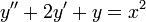$y''+2y'+y=x^2$ as an example.

Solve the homogeneous equation ( 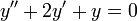$y''+2y'+y=0$ ) and get the roots of the characteristic equation ( $(m+1)^2=0, m=-1$ ) .
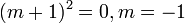Plug the roots into the general solution ( $y_c=c_1 sin(x)+c_2 cos(x)$ ) to obtain the complementary (homogeneous) solution.
To get the typical (specific) solution to the differential equation, we need to choose a "solution" from a table.
1. $1$ (any constant): $A$
2. $5x+7$ : $Ax+B$
3. $3x^2-2$ : $Ax^2+Bx+C$
4. $x^3-x+1$ : $Ax^3+Bx^2+Cx+D$
5. $sin(4x)$ : $A cos(4x)+B sin(4x)$
6. $cos(4x)$ : $A cos(4x)+B sin(4x)$
7. $e^{5x}$ : $Ae^{5x}$
8. $(9x-2)e^{5x}$ : $(Ax+B)e^{5x}$
9. $x^{2}e^{5x}$ : $(Ax^2+Bx+C)e^{5x}$
10. $e^{3x}sin(4x)$ : $Ae^{3x} cos(4x)+Be^{3x} sin(4x)$
11. $5x^{2}sin(4x)$ : $(Ax^2+Bx+C)cos(4x)+(Ex^2+Fx+G)sin(4x)$
12. $xe^{3x}cos(4x)$ : $(Ax+B)e^{3x} cos(4x)+(Cx+E)e^{3x} sin(4x)$
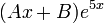
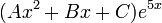
Choose the "solution" that best fits the right hand side of the equation. (the solution of $\textstyle x^2$ must take the form $\textstyle y_p = Ax^2+Bx+C$ ).
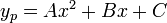Differentiate the "solution" to get the derivatives of the solution ( $y_p^{'}=2Ax+B, y_p^{''}=2A$ ).
Substitute those solutions into the left hand side of the original differential equation ( $(2A)+2(2Ax+B)+(Ax^2+Bx+C)=x^2$ ).
Collect and compare like terms to solve for the coefficients ( $A=1, B=-4, C=6$ ).
Substitute the coefficients back into typical "solution" ( $y_p=x^2-4x+6$ ).
Add the typical and the complementary solutions to get the complete solution ( $y=y_c+y_p=c_1 cos(x)+c_2 sin(x)+x^2 -4x+6$ ).

Variation of Parameters

Definition

Solution

This technique involves solving the complementary equation and using both solutions ( $y_1$ and $y_2$ ) as a basis to solve for two more particular solutions that combine to form the typical solution $y_p=u_1(x)+u_2(x)$ . To illustrate, let's solve the differential equation $y''-2y'-1=2xe^{3x}$ .

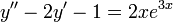Solve for the complementary solution ( $(m-1)^2=0, m=\pm 1, y_c=e^x+xe^x$ ).
Take each term in the complementary solution and make them separate functions ( $y_1=e^x, y_2=xe^x$ ).
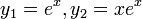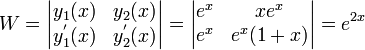
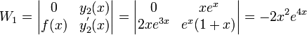
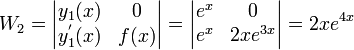
Set up the following three Wronksian matrices and take the determinants of them:
1. $W=\begin{vmatrix} y_1(x) & y_2(x) \\ y_1^{'}(x) & y_2^{'}(x) \end{vmatrix}=\begin{vmatrix} e^x & xe^x \\ e^x & e^x(1+x) \end{vmatrix}=e^{2x}$
2. $W_1=\begin{vmatrix} 0 & y_2(x) \\ f(x) & y_2^{'}(x) \end{vmatrix}=\begin{vmatrix} 0 & xe^x \\ 2xe^{3x} & e^x(1+x) \end{vmatrix}=-2x^2e^{4x}$
3. $W_2=\begin{vmatrix} y_1(x) & 0 \\ y_1^{'}(x) & f(x) \end{vmatrix}=\begin{vmatrix} e^x & 0 \\ e^x & 2xe^{3x} \end{vmatrix}=2xe^{4x}$
Solve for the terms 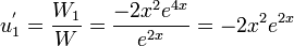$u_1^{'}=\frac {W_1}{W}=\frac {-2x^2e^{4x}}{e^{2x}}=-2x^2e^{2x}$ and $u_2^{'}=\frac {W_2}{W}=\frac {2xe^{4x}}{e^{2x}}=2xe^{2x}$ .
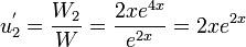Integrate them to get the terms 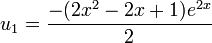$u_1=\frac {-(2x^2-2x+1)e^{2x}}{2}$ and $u_2=\frac {(2x-1)e^{2x}}{2}$ .
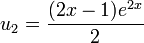Combine them with the complementary solution to get the complete solution ( $y=y_c+y_p=c_1 e^x+c_2 xe^x-\frac {(2x^2-2x+1)e^{2x}}{2}+\frac {(2x-1)e^{2x}}{2}$ ) .

This article is issued from Wikiversity - version of the Saturday, July 09, 2011. The text is available under the Creative Commons Attribution/Share Alike but additional terms may apply for the media files.