Kinematics
Introduction
- Kinematics
- Displacements, strains and the relations between displacements and strains.
- We view the theory of infinitesimal linear deformations as a first-order approximation of the theory of finite deformations.
- Note that the linear theory can be derived independently of the finite theory and is completely self-consistent on its own.
Concepts and Definitions
The following concepts and definitions are based on Gurtin (1972) and Truesdell and Noll (1992). These definitions are useful both for the linear and the nonlinear theory of elasticity.
Body
We usually denote a body by the symbol  . A body is essentially a set of points in Euclidean space. For mathematical definition see Truesdell and Noll (1992)
Configuration
A configuration of a body is denoted by the symbol  . A configuration of a body is just what the name suggests. Sometimes a configuration is also referred to as a placement.
Mathematically, we can think of a configuration as a smooth one-to-one mapping of a body into a region of three-dimensional Euclidean space.
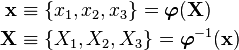
Thus, we can have a reference configuration  and a current configuration
  .
.
A one-to-one mapping is also called a homeomorphism.
Deformation
A deformation is the relationship between two configurations and is usually denoted by  . Deformations include both volume and shape changes and rigid body motions.
For a continuous body, a deformation can be thought of as a smooth mapping from one configuration ( ) to another (
 ). The inverse mapping should be possible.
This means that
For the inverse mapping to exist, we require that the Jacobian of the deformation is positive, i.e.,
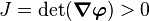 .
.
Deformation Gradient
The deformation gradient is usually denoted by  and is defined as

In index notation

For a deformation to be allowable, we must be able to invert . That is why we require that  . Otherwise, the body may undergo deformations that are unphysical.
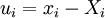
Displacement
The displacement is usually denoted by the symbol  .
.
The displacement is defined as a vector from the location of a material point in one configuration to the location of the same material point in another configuration.
The definition is

In index notation
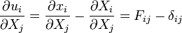
Displacement Gradient
The gradient of the displacement is denoted by
 .
.
The displacement gradient is given by

In index notation,
Strains
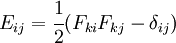
Finite Strain Tensor
The finite strain tensor ( ) is also called the Green-St. Venant Strain Tensor or the Lagrangian Strain Tensor.
This strain tensor is defined as
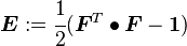
In index notation,
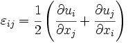
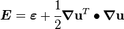
Infinitesimal Strain Tensor
In the limit of small strains, the Lagrangian finite strain tensor reduces to the infinitesimal strain tensor ( ).
).
This strain tensor is defined as
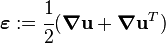
In index notation,
Therefore we can see that the finite strain tensor and the infinitesimal strain tensor are related by
If  , then

For small strains,  and
and
 .
.
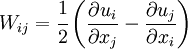
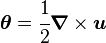
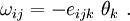
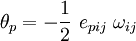
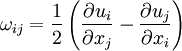
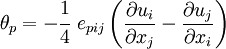
Infinitesimal Rotation Tensor
For small deformation problems, in addition to small strains we can also have small rotations ( ). The infinitesimal rotation tensor is defined as
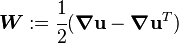
In index notation,
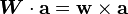
If  is a skew-symmetric tensor, then for any vector
  we have
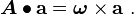
The vector  is called the axial vector of the skew-symmetric tensor.
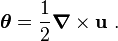
In our case,  is the skew-symmetric infinitesimal rotation tensor. The corresponding axial vector is the rotation vector
  defined as

where
Volume Change Due To Finite Deformation
The change in volume ( ) during a finite deformation is given by
Volume Change Due To Infinitesimal Deformation
The volume change during an infinitesimal deformation () is given by
because

The quantity  is called the dilatation.
A volume change is isochoric (volume preserving) if
 .
.
|
Let Let |
 be a displacement field. The displacement gradient tensor
is given by
be a displacement field. The displacement gradient tensor
is given by  . Let the skew symmetric part of the displacement
gradient tensor (infinitesimal rotation tensor) be
. Let the skew symmetric part of the displacement
gradient tensor (infinitesimal rotation tensor) be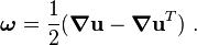
Proof:
The axial vector  of a skew-symmetric tensor satisfies the
condition
of a skew-symmetric tensor satisfies the
condition
for all vectors  . In index notation (with respect to a Cartesian
basis), we have
. In index notation (with respect to a Cartesian
basis), we have
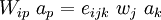
Since  , we can write

or,
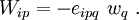
Therefore, the relation between the components of and
is
Multiplying both sides by  , we get

Recall the identity

Therefore,

Using the above identity, we get

Rearranging,
Now, the components of the tensor with respect to a Cartesian
basis are given by
Therefore, we may write
Since the curl of a vector  can be written in index notation as
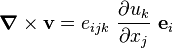
we have
![e_{pij}~\frac{\partial u_j}{\partial x_i}~ = [\boldsymbol{\nabla} \times \mathbf{u}]_p
\qquad \text{and} \qquad
e_{pij}~\frac{\partial u_i}{\partial x_j}~ = - e_{pji}\frac{\partial u_i}{\partial x_j} =
- [\boldsymbol{\nabla} \times \mathbf{u}]_p](../I/m/2ce6fa79df121e5c562839a18421b9d1.png)
where ![[~]_p](../I/m/a5e06e4f229ed997d83cda1e95a682c7.png) indicates the
indicates the  -th component of the vector inside the
square brackets.
-th component of the vector inside the
square brackets.
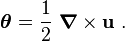
Hence,
![\theta_p = -\cfrac{1}{4}~\left(-[\boldsymbol{\nabla} \times \mathbf{u}]_p - [\boldsymbol{\nabla} \times \mathbf{u}]_p\right)
= \frac{1}{2}~[\boldsymbol{\nabla} \times \mathbf{u}]_p ~.](../I/m/af51434d0b8dc2bad56312356d13f477.png)
Therefore,
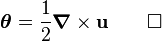
|
Let |
 be the strain field
(infinitesimal) corresponding to the displacement field and let
be the strain field
(infinitesimal) corresponding to the displacement field and let
Proof:
The infinitesimal strain tensor is given by
Therefore,
![\boldsymbol{\nabla} \times \boldsymbol{\varepsilon} = \frac{1}{2}[\boldsymbol{\nabla} \times (\boldsymbol{\nabla}\mathbf{u}) + \boldsymbol{\nabla} \times (\boldsymbol{\nabla}\mathbf{u}^T)] ~.](../I/m/cf81990d612f626e2dfb00db5bf653ba.png)
Recall that

Hence,
![\boldsymbol{\nabla} \times \boldsymbol{\varepsilon} = \frac{1}{2}[\boldsymbol{\nabla} (\boldsymbol{\nabla} \times \mathbf{u})] ~.](../I/m/a062cc69fc3ba9c137a335b7dcd072f2.png)
Also recall that
Therefore,

Related Content
- Introduction to Elasticity
- Help:Example template