Introduction to finite elements/Weighted residual methods
< Introduction to finite elementsWeak Formulation : Weighted Average Methods
Weighted average methods are also often called "Rayleigh-Ritz Methods". The idea is to satisfy the differential equation in an average sense by converting it into an integral equation. The differential equation is multiplied by a weighting function and then averaged over the domain.
If  is a weighting function then the weak form of Equation (1) is
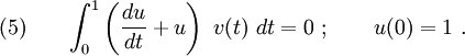
The weighting function can be any function of the independent variables that is sufficiently well-behaved that the integrals make sense.
Recall that we are looking for an approximate solution. Let us call this approximate solution  . If we plug the approximate solution into equation (5) we get

Since the solution is approximate, the original differential equation will not be satisfied exactly and we will be left with a residual  . Weighted average methods try to minimize the residual in a weighted average sense.
Finite element methods are a special type of weighted average method.
Examples of Weighted Average Methods
Let us assume the trial solution for problem (6) to be

After applying the initial condition we get  , and the trial solution becomes

Let us simplify the trial solution further and consider only the first three terms, i.e.,

Plug in the trial solution (7) into (6). Then, the residual is

If  , then the trial solution is equal to the exact solution. If
  , we can try to make the residual as close to zero as possible. This can be done by choosing
  and
and  such that is a minimum.
Minimizing : Collocation Method
In the collocation method, we minimize the residual by making it vanish at  points
  within the domain.
For our problem, the domain of interest is  . Let us pick two points in this domain
  and
and  such that
  (see Figure 1). In this example we choose
  and
and  .
.
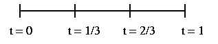 Figure 1. Discretized domain for Problem 1. |
The values of the residual (8) at and are

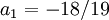
If we now impose the condition that the residual vanishes at these two points and solve the resulting equations, we get  and
and  .
Therefore the approximate solution is
.
Therefore the approximate solution is
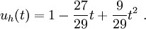
Figure 2 shows a comparison of this solution with the exact solution.
You can see that the collocation method gives a solution that is close to the exact up to  . However, the same results cannot be used up to
  without re-evaluating the integrals.
If you think in terms of equation (6) you can see that a weighting function was used to get to the solution. In fact, it is the choice of weighting function that determines whether a method is a collocation method! The weighting function in this case is
where  is a node and
  is the Dirac delta function.
Minimizing : Subdomain Method
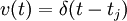
The subdomain method is another way of minimizing the residuals. In this case, instead of letting the residual vanish at unique points, we let the "average" of the residual vanish over each domain. That is, we let,
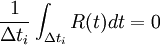
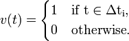
where  is the subdomain over which averaging is done. From this definition it is clear that the weighting function for the subdomain method is
Let us apply the subdomain method to Problem 1. We discretize the domain by choosing one point between  and
and  at
at  . For the two subdomains (elements) we have,

Setting these residuals to zero and solving for and we get
 and
and  . Therefore the approximate solution is
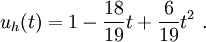
Figure 2 shows a comparison of the exact solution and the subdomain and the collocation solutions.
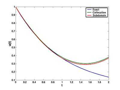 Figure 2. Subdomain solution versus exact solution for Problem 1. |
Minimizing : Galerkin Method
In this case, instead of writing our trial function as,

we write it as
where  are
are  linearly independent functions of
  . These are called basis functions, interpolation functions, or shape functions. The first term
  is left outside the sum because it is associated with part or all of the initial or boundary conditions (i.e., we put everything that can be fixed by initial or boundary conditions into ).
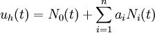
Then the trial function in equation (7) can be rewritten using basis functions as

where

Important:
In the Galerkin method we choose the basis functions  as the weighting functions.
If we use  as the weighting functions , equation (6) becomes

Plugging in the value of from equation (8) into equation (13) and using the basis functions from (12) we get
![\int^1_0 \left[ 1 + a_1(1+t) + a_2(2t + t^2)\right]~t~dt = 0
\quad\text{and}\quad
\int^1_0 \left[ 1 + a_1(1+t) + a_2(2t + t^2)\right]~t^2~dt = 0~.](../I/m/89fb1b9ba9bced2c6ac4e396b377c04d.png)
After integrating and solving for and we get  and
and  . Therefore, the Galerkin approximation we seek is
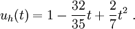
Figure 3 shows a comparison of the exact solution with the Galerkin, subdomain, and collocation solutions.
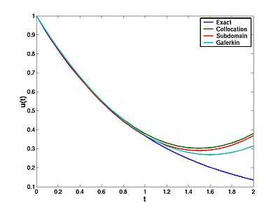 Figure 3. Galerkin solution versus exact solution for Problem 1. |
All the approximate solutions diverge from the exact solution beyond . The solution to this problem is to break up the domain into elements so that the trial solution is a good approximation to the exact solution in each element.
Minimizing : Least Squares Method
In the least-squares method, we try to minimize the residual in a least-squares sense, that is

where  . The weighting function for the least squares method is therefore
Plugging in the value of from equation (8) into equation (15) and using the basis functions from (12) we get
![\int^1_0 \left[ 1 + a_1(1+t) + a_2(2t + t^2)\right]~(1+t)~dt = 0
\quad\text{and}\quad
\int^1_0 \left[ 1 + a_1(1+t) + a_2(2t + t^2)\right]~(2t+t^2)~dt = 0~.](../I/m/f9db398b50d6de88df4c2bde8b05bc17.png)
After integrating and solving for and we get  and
and 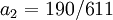 . Therefore, the least squares approximation we seek is
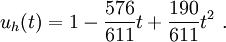
Figure 4 shows a comparison of the exact solution with the Galerkin, subdomain, and collocation solutions.
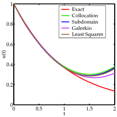 Figure 4. Least squares solution versus other solutions for Problem 1. |