Introduction to finite elements/Model problems

Model problems

Let us look at a couple of model problems.

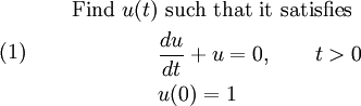
Problem 1: First-order homogeneous ODE

The first problem involves a homogeneous first order differential equation and is stated as:

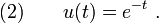
\text{(1)} \qquad { \begin{align} \text{Find}~ u(t) & ~\text{such that it satisfies} \\ & \frac{du}{dt} + u = 0, \qquad t > 0 \\ & u(0) = 1 \end{align} }

The exact solution is

\text{(2)} \qquad { u(t) = e^{-t}~. }

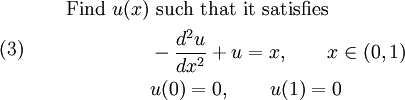
Problem 2: Second-order inhomogeneous ODE

The second problem involves an inhomogeneous second order differential equation and is stated as:

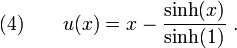
\text{(3)} \qquad { \begin{align} \text{Find}~ u(x) & ~\text{such that it satisfies} \\ & -\frac{d^2u}{dx^2} + u = x, \qquad x \in (0,1) \\ & u(0) = 0, \qquad u(1) = 0 \end{align} }

The exact solution is

\text{(4)} \qquad { u(x) = x - \frac{\sinh(x)}{\sinh(1)} ~. }

Remarks

Both model problems have exact solutions. However, in most situations, such solutions may be impossible to get because:

No solution exists since the data are not smooth enough.
Even if a solution exists, it cannot be found in closed form because of the complexity of the problem.

To overcome these problems, we can do the following :

Reformulate the problem so that it admits weaker conditions on the solution and its derivatives. Thus the equation no longer needs to be satisfied at all points in the domain. These are called weak or variational formulations.
Break the domain up into smaller pieces and require the equation to be satisfied at only a few points within each piece.
Assume that the approximate solution has a known form.

Finite element methods use a weak (or variational) formulation of the original strong problem.

This article is issued from Wikiversity - version of the Thursday, November 22, 2007. The text is available under the Creative Commons Attribution/Share Alike but additional terms may apply for the media files.