Introduction to finite elements/Model finite element approximation

Finite Element Formulation for Problem 2.

The domain for this problem is $\Omega = \{x ~|~ x \in (0,1)\}$ and the boundary consists of two points $\Gamma = \{0,1\}$ . Let us use $n$ nodes in the domain so that they divide the domain into $n-1$ nonoverlapping, two-noded elements.

Consider the term $K_{ij}$ in equation (22). The integral can be written as a sum of integrals over each element as

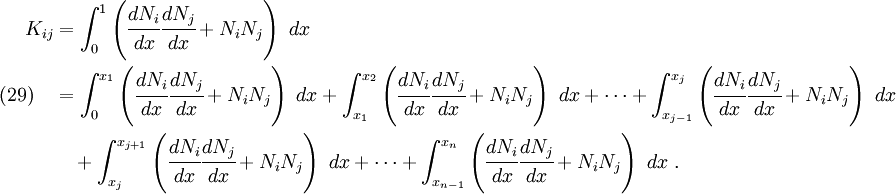
\begin{align} K_{ij} & = \int^1_0 \left(\cfrac{dN_i}{dx} \cfrac{dN_j}{dx} + N_i N_j \right)~dx \\ \text{(29)} \quad & = \int_0^{x_1}\left(\cfrac{dN_i}{dx}\cfrac{dN_j}{dx}+N_i N_j\right)~dx+ \int_{x_1}^{x_2}\left(\cfrac{dN_i}{dx}\cfrac{dN_j}{dx}+N_i N_j\right)~dx+ \dots + \int_{x_{j-1}}^{x_j}\left(\cfrac{dN_i}{dx}\cfrac{dN_j}{dx}+N_i N_j\right) ~dx \\ & ~~~ + \int_{x_{j}}^{x_{j+1}}\left(\cfrac{dN_i}{dx}\cfrac{dN_j}{dx}+N_i N_j\right) ~dx+ \dots + \int_{x_{n-1}}^{x_n}\left(\cfrac{dN_i}{dx}\cfrac{dN_j}{dx}+N_i N_j\right) ~dx~. \end{align}

In this equation, $i$ and $j$ are node numbers. Therefore there are $n \times n$ possible values of $K_{ij}$ .

Assume that node $i$ = 2 and node $j$ = 4. Then $N_i = 1$ at node 2 and zero at all the other nodes. Similarly, $N_j = 1$ at node 4 and zero at all other nodes. Also, $N_i$ is non-zero only between nodes 1, 2, and 3 while $N_j$ is nonzero only between nodes 3, 4, and 5. Since the domains of $N_i$ and $N_j$ do not overlap in this case, all the integrals must be zero.

In general, if $i$ and $j$ are separated by more than one node, at least one of the basis functions has a zero value within each integral. The same holds for the derivatives of the basis functions. Therefore $K_{ij} = 0$ if $i$ and $j$ are separated by more than one node.

Therefore, there are three non-trivial cases that need to be looked at

$i = j$ .
$i = j-1$ .
$i = j+1$ .

For the first case, set $i = j$ in equation (29). That means

\text{(30)} \qquad \int_0^1 \left(\cfrac{dN_j}{dx}\cfrac{dN_j}{dx} + N_j N_j\right)~ dx = \int_{x_{j-1}}^{x_{j}} \left(\cfrac{dN_j}{dx}\cfrac{dN_j}{dx} + N_j N_j\right) ~dx + \int_{x_{j}}^{x_{j+1}} \left(\cfrac{dN_j}{dx}\cfrac{dN_j}{dx} + N_j N_j\right) ~dx ~.

After substituting the values of the basis functions (25) and their derivatives (26) into equation (30) and integrating, we get

{ K_{jj} = \int_0^1 \left(\cfrac{dN_j}{dx}\cfrac{dN_j}{dx} + N_j N_j\right)~ dx = \cfrac{1}{x_j - x_{j-1}} + \cfrac{1}{x_{j+1} - x_j} + \cfrac{x_{j+1} - x_{j-1}}{3} ~. }

For the second case, set $i = j-1$ in equation (29). In this case, the only non-zero integrals in equation (29) are the ones between $x_{j-1}$ and $x_j$ . Hence

\text{(31)} \qquad \int_0^1 \left(\frac{dN_{j-1}}{dx}\frac{dN_j}{dx} + N_{j-1} N_j\right)~dx = \int_{x_{j-1}}^{x_j} \left(\frac{dN_{j-1}}{dx}\frac{dN_j}{dx} + N_{j-1} N_j\right)~ dx~.

After substituting the basis functions and their derivatives into equation (31) and integrating, we get

{ K_{(j-1)j} = \int_0^1 \left(\frac{dN_{j-1}}{dx}\frac{dN_j}{dx} + N_{j-1} N_j\right)~dx = - \frac{1}{x_j - x_{j-1}} + \frac{x_{j} - x_{j-1}}{6} ~. }

For the third case, set $i = j+1$ in equation (29). In this case, the only non-zero integrals in equation (29) are the ones between $x_j$ and $x_{j+1}$ . Hence

\text{(32)} \qquad \int_0^1 \left(\frac{dN_j}{dx}\frac{dN_{j+1}}{dx} + N_j N_{j+1}\right)~dx = \int_{x_j}^{x_{j+1}} \left(\frac{dN_j}{dx}\frac{dN_{j+1}}{dx} + N_j N_{j+1}\right)~ dx~.

After substituting the basis functions and their derivatives into equation (\ref{eq:Integralij+1}) and integrating, we get

{ K_{j(j+1)} = \int_0^1 \left(\frac{dN_j}{dx}\frac{dN_{j+1}}{dx} + N_j N_{j+1}\right)~dx = - \frac{1}{x_{j+1} - x_j} + \frac{x_{j+1} - x_j}{6} ~. }

The same process can be followed for the integral

{ f_j = \int^1_0 x~ N_j~ dx = \int_{x_{j-1}}^{x_j} x~N_j~dx + \int_{x_j}^{x_{j+1}} x~N_j~dx = \cfrac{2 x_j^3 - 3 x_j^2 x_{j-1} + x_{j-1}^3}{6(x_j - x_{j-1})} + \cfrac{2 x_j^3 - 3 x_j^2 x_{j+1} + x_{j+1}^3}{6(x_{j+1} - x_j)} ~. }

Now that we know the components $K_{ij}$ and $f_j$ , we can solve the system of equations (23) for the unknowns $a_i$ . This gives us our finite element solution for Problem 2.

Assembly process.

In the above we did not go through the assembly process that you are familiar with from introductory finite elements. We can simplify things if we use just compute the integrals over each element and assemble them to get the final $\mathbf{K}$ and $\mathbf{f}$ matrices.

To see how the assembly process works, let us recall equation (21)

\text{(33)} \qquad { \sum_{i=1}^n a_i \int^1_0 \left(\cfrac{dN_i}{dx} \cfrac{dN_j}{dx} + N_i N_j\right)~dx - \int^1_0 x~N_j~dx = 0 \qquad j = 1\dots n~. }

We can rewrite this equation as

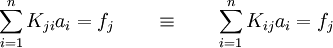
\sum_{i=1}^n K_{ji} a_i = f_j \qquad \equiv \qquad \sum_{i=1}^n K_{ij} a_i = f_j

where

\text{(34)} \qquad K_{ij} = a(N_i,N_j) = \int^1_0 \left(\cfrac{dN_i}{dx} \cfrac{dN_j}{dx} + N_i N_j\right)~dx \qquad \text{and} \qquad f_j = \langle x,N_j\rangle = \int^1_0 x~N_j~dx ~.

Let us define

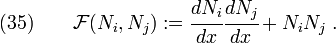
\text{(35)} \qquad \mathcal{F}(N_i,N_j) := \cfrac{dN_i}{dx} \cfrac{dN_j}{dx} + N_i N_j ~.

Then the first of the equations in (34) can be written as

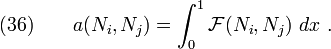
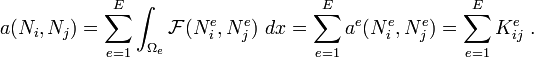
\text{(36)} \qquad a(N_i,N_j) = \int^1_0 \mathcal{F}(N_i,N_j) ~dx ~.

From equation (29) we can see that the integral over the entire domain $\Omega$ can be written as a sum of integrals over the elements $\Omega_e$ . Therefore, we can write equation (36) as

\text{(37)} \qquad a(N_i,N_j) = \int_{\Omega} \mathcal{F}(N_i,N_j) ~dx = \sum_{e=1}^E \int_{\Omega_e} \mathcal{F}(N_i,N_j) ~dx ~.

Let $N_i^e$ be the local basis functions in an element. Then equation (37) can be written as

a(N_i,N_j) = \sum_{e=1}^E \int_{\Omega_e} \mathcal{F}(N_i^e,N_j^e) ~dx = \sum_{e=1}^E a^e(N_i^e,N_j^e) = \sum_{e=1}^E K^e_{ij} ~.

Similarly, the second equation in (34) can be written as

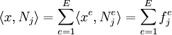
\langle x,N_j \rangle = \sum_{e=1}^E \langle x^e,N_j^e \rangle = \sum_{e=1}^E f^e_j

where $x^e$ indicates that the integral is over the element.

Therefore, the matrix $\mathbf{K}$ and the vector $\mathbf{f}$ can be expressed as a sum over the elements in the form

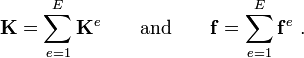
\mathbf{K} = \sum_{e=1}^E \mathbf{K}^e \qquad \text{and} \qquad \mathbf{f} = \sum_{e=1}^E \mathbf{f}^e ~.

This is the familiar assembly process. From this process it is clear that if we can find the weak form for one element, then the finite element system of equations for any combination of such elements can be computed by assembly.

This article is issued from Wikiversity - version of the Thursday, August 16, 2007. The text is available under the Creative Commons Attribution/Share Alike but additional terms may apply for the media files.