Introduction to finite elements/Choosing weight function

Choice of Weighting Functions

As you have seen, we need to know the weighting functions (also called test functions) in order to define the weak (or variational) statement of the problem more precisely.

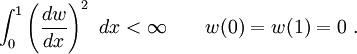
Consider the second model problem (3). If $w(x)$ is a weighting function, then the weak form of equation (3) is

\text{(17)} \qquad { \int^1_0 \left[-\frac{d^2}{dx^2}[u(x)] + u(x) - x\right]~w(x)~dx= 0 }

Let the possible weighting functions $w(x)$ for this equation be such that they satisfy the boundary conditions, that is $w(0) = 0$ and $w(1) = 0$ . This set of weighting functions will be denoted by the symbol $\mathcal{H}$ .

The exact weak form of the problem can then be stated as:

 $\begin{align} \text{Find}~ u(x)~& ~\text{such that} \\ & \int^1_0 \left[-\frac{d^2}{dx^2}[u(x)] + u(x) - x\right] w(x) ~dx \qquad \text{for all} ~ w(x) \in \mathcal{H} \\ & u(0) = 0, u(1) = 0 ~;~~ \qquad w(0) = 0, w(1) = 0 ~. \end{align}$

To get to an approximate weak form, we need to choose trial functions. Let these trial functions ( $u_h$ ) reside in the function space $\mathcal{S}$ . The approximate weak form of the problem is

 $\begin{align} \text{Find}~ u_h(x) \in \mathcal{S} ~& ~\text{such that} \\ & \int^1_0 \left[-\frac{d^2}{dx^2}[u_h(x)] + u_h(x) - x\right] w(x) ~dx \qquad \text{for all} ~ w(x) \in \mathcal{H} \\ & u_h(0) = 0, u_h(1) = 0 ~;~~ \qquad w(0) = 0, w(1) = 0 ~. \end{align}$

One requirement that these trial functions ( $u_h$ ) have to satisfy is that

\int_0^1 \left(\cfrac{d^2u_h}{dx^2}\right) w(x)~dx < \infty ~.

The trial functions also have to satisfy the boundary conditions.

If you look at the weak form shown above, you will notice that the highest derivatives of $u_h$ are of the second order while there are no derivatives of $w$ . This leads to a lack of symmetry in the formulation that is usually avoided for numerical reasons.

To get a symmetric weak form, we integrate the first term inside the integral by parts to get

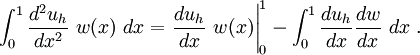
\int^1_0 \frac{d^2u_h}{dx^2}~w(x)~dx = \left.\frac{du_h}{dx}~w(x) \right|^1_0 - \int^1_0 \frac{du_h}{dx} \frac{dw}{dx}~ dx ~.

(Recall that the formula for integration by parts is 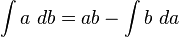$\int a~db = ab - \int b~da$ .)

Applying the boundary conditions on $w(x)$ , we get

\int^1_0 \frac{d^2u_h}{dx^2}~w(x)~dx = - \int^1_0 \frac{du_h}{dx} \frac{dw}{dx}~ dx ~.

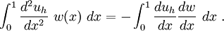
Therefore the problem can be restated in symmetric form as :

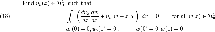
 $\text{(18)} \qquad \begin{align} \text{Find}~ u_h(x) \in \mathcal{H}^1_0 ~& ~\text{such that} \\ & \int^1_0 \left(\frac{du_h}{dx}\frac{dw}{dx} + u_h~w - x~w\right)~dx = 0 \qquad ~\text{for all}~ w(x) \in \mathcal{H}^1_0 \\ & u_h(0) = 0, u_h(1) = 0 ~;~~ \qquad w(0) = 0, w(1) = 0 \end{align}$

Since the same order of derivatives appear in both the trial and the weighting functions, we can choose our functions from the same set 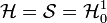$\mathcal{H}^1_0$ , where $\mathcal{H} = \mathcal{S} = \mathcal{H}^1_0$ . As you can see, the smoothness requirements on $w$ are further weakened. This boundary value problem is also called the variational boundary value problem.

The variational boundary value problem (18) can be (and often is) written using bilinear function notation as

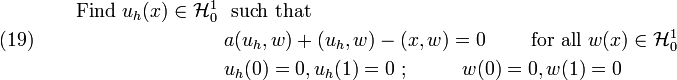
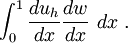
 $\text{(19)} \qquad \begin{align} \text{Find}~ u_h(x) \in \mathcal{H}^1_0 ~& ~\text{such that} \\ & a(u_h, w) + (u_h, w) - (x,w) = 0 \qquad ~\text{for all}~ w(x) \in \mathcal{H}^1_0 \\ & u_h(0) = 0, u_h(1) = 0 ~;~~ \qquad w(0) = 0, w(1) = 0 \end{align}$

where

{ a(u_h,w) = \int^1_0 \frac{du_h}{dx}\frac{dw}{dx}~dx ~;\qquad (u_h,w) = \int_0^1 u_h~w~dx ~; \qquad (x,w) = \int_0^1 x~w~dx ~. }

Characteristics of $\mathcal{H}^1_0$

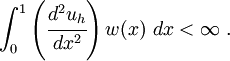
Let us now characterize $\mathcal{H}^1_0$ , the class of admissible functions for the problem. We know that if $u_h$ and $w$ are irregular then their derivatives are even more irregular. Therefore, the most irregular term in the problem statement is

\int_0^1 \frac{du_h}{dx} \frac{dw}{dx}~dx ~.

Now, both $u_h$ and $w$ are functions in the space $\mathcal{H}^1_0$ . So we can choose $w$ to be equal to $u_h$ . Hence the minimum requirement for $w$ is

{ \int_0^1\left(\frac{dw}{dx}\right)^2~dx < \infty \qquad w(0) = w(1) = 0~. }

Functions like the above are called square integrable.

Thus, our weighting functions have to be square integrable. This is a stricter condition than just requiring $w$ to be piecewise continuous, and reduces the number of functions that you can choose from.

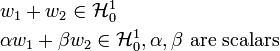
There are two other interesting properties of the space $\mathcal{H}^1_0$ . These are :

It is a linear space which means that if $w_1$ and $w_2$ are two arbitrary functions in this space, then the following operations hold :

\begin{align} & w_1 + w_2 \in \mathcal{H}^1_0 \\ & \alpha w_1 + \beta w_2 \in \mathcal{H}^1_0, \alpha, \beta ~\text{are scalars} \end{align}

It is an infinite dimensional space. This means that an infinity of parameters are needed to uniquely determine a weighting function $w~\in\mathcal{H}^1_0$ . Thus,

w(x) = \sum^{\infty}_{i=1} a_i N_i(x)

where,

N_i

are linearly independent functions (also called basis functions) and

a_i

are constants. If we choose only

n

of these basis functions

\{N_1, N_2, \dots, N_n\}

then this is a

n

-dimensional (i.e., finite dimensional) subspace of

\mathcal{H}^1_0

and we denote this as

\mathcal{H}^n_0

This article is issued from Wikiversity - version of the Thursday, August 16, 2007. The text is available under the Creative Commons Attribution/Share Alike but additional terms may apply for the media files.