Introduction to finite elements/Axial bar finite element solution
< Introduction to finite elementsAxially loaded bar: The Finite Element Solution
The finite element method is a type of Galerkin method that has the following advantages:
- The functions
 are found in a systematic manner.
 - The functions are chosen such that they can be used for arbitrary domains.
- The functions are piecewise polynomials.
- The functions are non-zero only on a small part of the domain.
As a result, computations can be done in a modular manner that is suitable for computer implementation.
Discretization
The first step in the finite element approach is to divide the domain into elements and nodes, i.e., to create the finite element mesh.
Let us consider a simple situation and divide the rod into 3 elements and 4 nodes as shown in Figure 6.
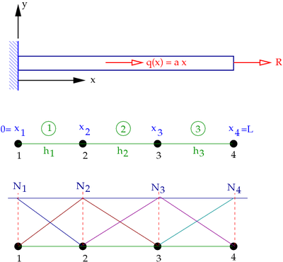 Figure 6. Finite element mesh and basis functions for the bar. |
Shape functions
The functions have special characteristics in finite element methods and are generally written as  and are called basis functions, shape functions, or interpolation functions.
Therefore, we may write
The finite element basis functions are chosen such that they have the following properties:
- The functions are bounded and continuous.
- If there are
 nodes, then there are basis functions - one for each node. There are four basis functions for the mesh shown in Figure 6.
 - Each function is nonzero only on elements connected to node
 .
. - is 1 at node and zero at all other nodes.
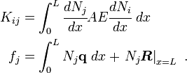
Stiffness matrix
Let us compute the values of  for the three element mesh. We have
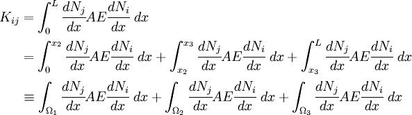
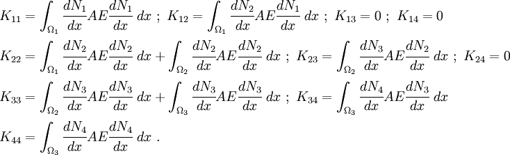
The components of  are
are
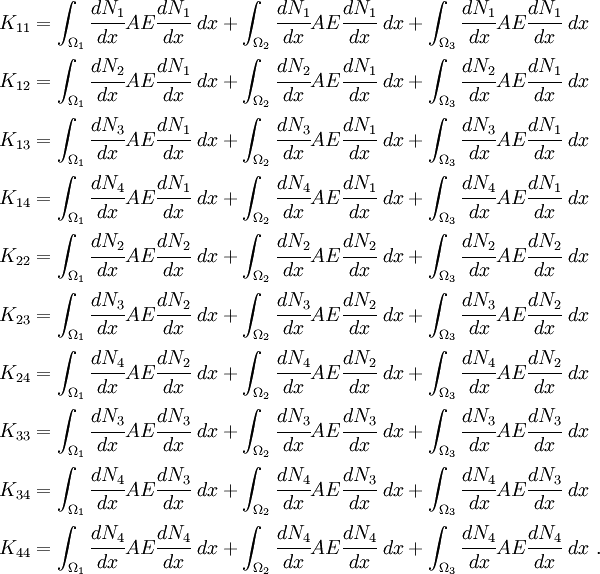
The matrix is symmetric, so we don't need to explicitly compute the other terms.
From Figure 6, we see that  is zero in elements 2 and 3,
  is zero in element 3,
  is zero in element 1, and
  is zero in elements 1 and 2. The same holds for
  .
.
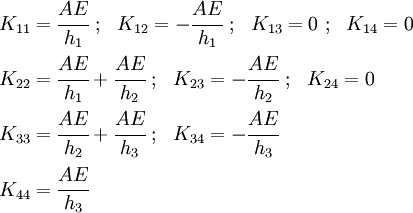
Therefore, the coefficients of the matrix become
We can simplify our calculation further by letting  be the shape functions over an element
  . For example, the shape functions over element
  are
are  and
and  where the local nodes
  and correspond to global nodes and
  , respectively. Then we can write,
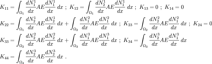
Let  be the part of the value of that is contributed by element . The indices
  are local and the indices
  are global. Then,
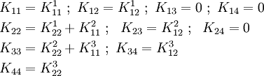
We can therefore see that if we compute the stiffness matrices over
each element and assemble them in an appropriate manner, we can get the
global stiffness matrix .
Stiffness matrix for two-noded elements
For our problem, if we consider an element with two nodes, the local hat shape functions have the form
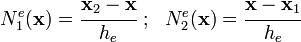
where  is the length of the element.
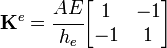
Then, the components of the element stiffness matrix are
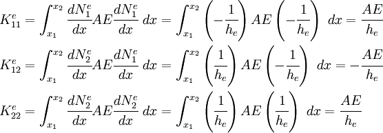
In matrix form,
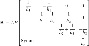
The components of the global stiffness matrix are
In matrix form,
Load vector
Similarly, for the load vector  , we have
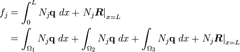
The components of the load vector are
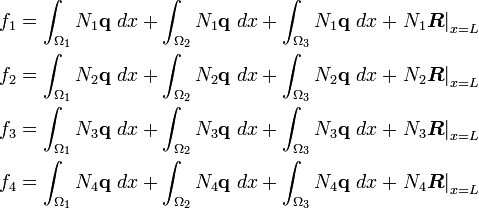
Once again, since is zero in elements 2 and 3, is zero in element 3, is zero in element 1, and is zero in elements 1 and 2, we have
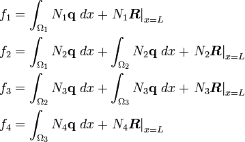
Now, the boundary  is at node 4 which is attached to element 3. The only non-zero shape function at this node is . Therefore, we have
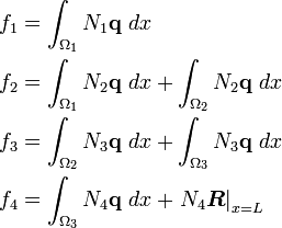
In terms of element shape functions, the above equations can be written as
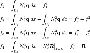
The above shows that the global load vector can also be assembled from the element load vectors if we use finite element shape functions.
Load vector for two-noded elements
Using the linear shape functions discussed earlier and replacing  with
with  , the components of the element load vector
  are
are
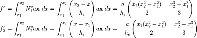
In matrix form, the element load vector is written
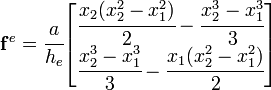
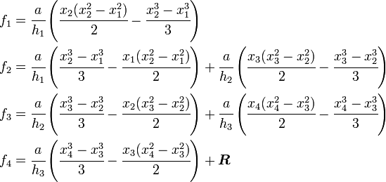
Therefore, the components of the global load vector are
Displacement trial function
Recall that we assumed that the displacement can be written as
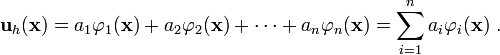
If we use finite element shape functions, we can write the above as
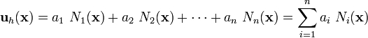
where is the total number of nodes in the domain. Also, recall that the value of is 1 at node and zero elsewhere. Therefore, we have
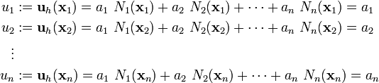
Therefore, the trial function can be written as
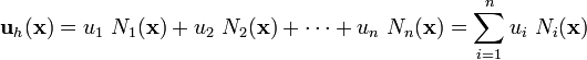
where  are the nodal displacements.
Finite element system of equations
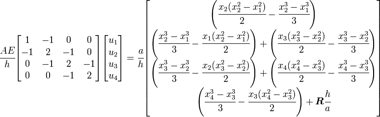
If all the elements are assumed to be of the same length  , the finite element system of equations (
 ) can then be written as
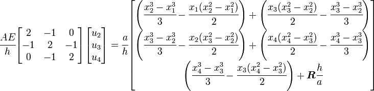
Essential boundary conditions
To solve this system of equations we have to apply the essential boundary condition  at
at  . This is equivalent to setting
  . The reduced system of equations is
This system of equations can be solved for  ,
,  , and
, and  . Let us do that.
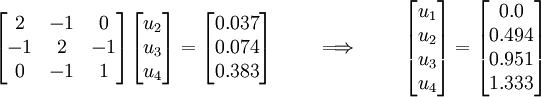
Assume that  ,
,  ,
,  ,
,  , and
, and  are all equal to 1. Then
  ,
,  ,
,  ,
,  , and
, and  . The system of equations becomes
Computing element strains and stresses
From the above, it is clear that the displacement field within an element is given by

Therefore, the strain within an element is
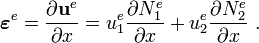
In matrix notation,
![\boldsymbol{\varepsilon}^e = \mathbf{B}^e \mathbf{u}^e
= \left[ \frac{\partial N^e_1}{\partial x} ~~ \frac{\partial N^e_2}{\partial x}\right]
\begin{bmatrix} u^e_1 \\ u^e_2 \end{bmatrix}
= \left[ -\cfrac{1}{h} ~~ \cfrac{1}{h} \right]
\begin{bmatrix} u^e_1 \\ u^e_2 \end{bmatrix}](../I/m/56b1f6cb64454c55ac81633f0a3fd445.png)
The stress in the element is given by

For our discretization, the element stresses are

A plot of this solution is shown in Figure 7.
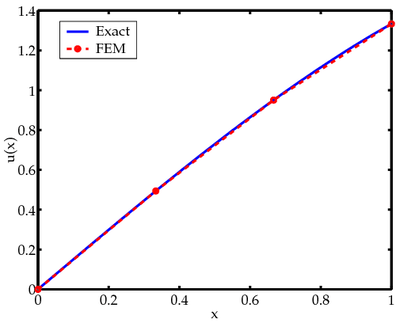 Figure 7(a). FEM vs exact solutions for displacements of an axially loaded bar. |
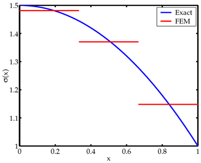 Figure 7(b). FEM vs exact solutions for stresses in an axially loaded bar. |
Matlab code
The finite element code (Matlab) used to compute this solution is given below.
    function AxialBarFEM

      A = 1.0;
      L = 1.0;
      E = 1.0;
      a = 1.0;
      R = 1.0;

      e = 3;
      h = L/e;
      n = e+1;
      for i=1:n
        node(i) = (i-1)*h;
      end
      for i=1:e
        elem(i,:) = [i i+1];
      end

      K = zeros(n);
      f = zeros(n,1);
      for i=1:e
        node1 = elem(i,1);
        node2 = elem(i,2);
        Ke = elementStiffness(A, E, h);
        fe = elementLoad(node(node1),node(node2), a, h);
        K(node1:node2,node1:node2) = K(node1:node2,node1:node2) + Ke;
        f(node1:node2) = f(node1:node2) + fe;
      end

      f(n) = f(n) + 1.0;

      Kred = K(2:n,2:n);
      fred = f(2:n);

      d = inv(Kred)*fred;

      dsol = [0 d'];

      fsol = K*dsol';
      sum(fsol)

      figure;
      p0 = plotDisp(E, A, L, R, a);
      p1 = plot(node, dsol, 'ro--', 'LineWidth', 3); hold on;
      legend([p0 p1],'Exact','FEM');

      for i=1:e
        node1 = elem(i,1);
        node2 = elem(i,2);
        u1 = dsol(node1);
        u2 = dsol(node2);
        [eps(i), sig(i)] = elementStrainStress(u1, u2, E, h);
      end

      figure;
      p0 = plotStress(E, A, L, R, a);
      for i=1:e
        node1 = node(elem(i,1));
        node2 = node(elem(i,2));
        p1 = plot([node1 node2], [sig(i) sig(i)], 'r-','LineWidth',3); hold on;
      end
      legend([p0 p1],'Exact','FEM');

    function [p] = plotDisp(E, A, L, R, a)

      dx = 0.01;
      nseg = L/dx;
      for i=1:nseg+1
        x(i) = (i-1)*dx;
        u(i) = (1/6*A*E)*(-a*x(i)^3 + (6*R + 3*a*L^2)*x(i));
      end
      p = plot(x, u, 'LineWidth', 3); hold on;
      xlabel('x', 'FontName', 'palatino', 'FontSize', 18);
      ylabel('u(x)', 'FontName', 'palatino', 'FontSize', 18);
      set(gca, 'LineWidth', 3, 'FontName', 'palatino', 'FontSize', 18);

    function [p] = plotStress(E, A, L, R, a)

      dx = 0.01;
      nseg = L/dx;
      for i=1:nseg+1
        x(i) = (i-1)*dx;
        sig(i) = (1/2*A*E)*(-a*x(i)^2 + (2*R + a*L^2));
      end
      p = plot(x, sig, 'LineWidth', 3); hold on;
      xlabel('x', 'FontName', 'palatino', 'FontSize', 18);
      ylabel('\sigma(x)', 'FontName', 'palatino', 'FontSize', 18);
      set(gca, 'LineWidth', 3, 'FontName', 'palatino', 'FontSize', 18);

    function [Ke] = elementStiffness(A, E, h)

      Ke = (A*E/h)*[[1 -1];[-1 1]];

    function [fe] = elementLoad(node1, node2, a, h)

      x1 = node1;
      x2 = node2;

      fe1 = a*x2/(2*h)*(x2^2-x1^2) - a/(3*h)*(x2^3-x1^3);
      fe2 = -a*x1/(2*h)*(x2^2-x1^2) + a/(3*h)*(x2^3-x1^3);
      fe = [fe1;fe2];

    function [eps, sig] = elementStrainStress(u1, u2, E, h)

      B = [-1/h 1/h];
      u = [u1; u2];
      eps = B*u
      sig = E*eps;