Introduction to finite elements/Axial bar approximate solution

Approximate Solution: The Galerkin Approach

To find the finite element solution, we can either start with the strong form and derive the weak form, or we can start with a weak form derived from a variational principle.

Let us assume that the approximate solution is $\mathbf{u}_h(\mathbf{x})$ and plug it into the ODE. We get

AE \cfrac{d^2\mathbf{u}_h}{dx^2} + a \mathbf{x} = R_h(\mathbf{x})

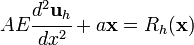
where $R_h$ is the residual. We now try to minimize the residual in a weighted average sense

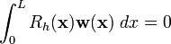
\int_0^L R_h(\mathbf{x}) \mathbf{w}(\mathbf{x}) ~dx = 0

where $\mathbf{w}(\mathbf{x})$ is a weighting function. Notice that this equation is similar to equation (5) (see 'Weak form: integral equation') with $\mathbf{w}$ in place of the variation $\delta \mathbf{u}$ . For the two equations to be equivalent, the weighting function must also be such that $\mathbf{w}(0) = 0$ .

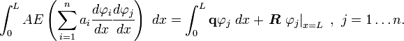
Therefore the approximate weak form can be written as

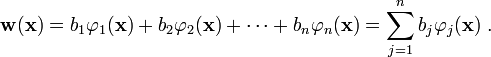
{ \int_0^L AE \cfrac{d\mathbf{u}_h}{dx}\cfrac{d\mathbf{w}}{dx}~dx = \int_0^L\mathbf{q}\mathbf{w}~dx + \left. \boldsymbol{R}~\mathbf{w}\right|_{x=L} ~. }

In Galerkin's method we assume that the approximate solution can be expressed as

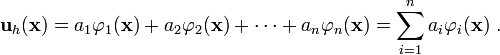
\mathbf{u}_h(\mathbf{x}) = a_1\varphi_1(\mathbf{x}) + a_2\varphi_2(\mathbf{x}) + \dots + a_n\varphi_n(\mathbf{x}) = \sum_{i=1}^n a_i \varphi_i(\mathbf{x}) ~.

In the Bubnov-Galerkin method, the weighting function is chosen to be of the same form as the approximate solution (but with arbitrary coefficients),

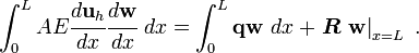
\mathbf{w}(\mathbf{x}) = b_1\varphi_1(\mathbf{x}) + b_2\varphi_2(\mathbf{x}) + \dots + b_n\varphi_n(\mathbf{x}) = \sum_{j=1}^n b_j \varphi_j(\mathbf{x}) ~.

If we plug the approximate solution and the weighting functions into the approximate weak form, we get

\int_0^L AE \left(\sum_{i=1}^n a_i\cfrac{d\varphi_i}{dx}\right) \left(\sum_{j=1}^n b_j\cfrac{d\varphi_j}{dx}\right)~dx = \int_0^L\mathbf{q}\left(\sum_{j=1}^n b_j\varphi_j\right)~dx + \left. \boldsymbol{R}~\left(\sum_{j=1}^n b_j\varphi_j\right)\right|_{x=L} ~.

This equation can be rewritten as

\sum_{j=1}^n b_j \left[\int_0^L AE \left(\sum_{i=1}^n a_i\cfrac{d\varphi_i}{dx} \cfrac{d\varphi_j}{dx}\right)~dx \right] = \sum_{j=1}^n b_j \left[\int_0^L\mathbf{q}\varphi_j~dx + \left. \left(\boldsymbol{R}~\varphi_j\right)\right|_{x=L}\right] ~.

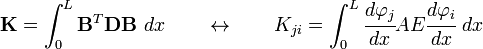
From the above, since $b_j$ is arbitrary, we have

\int_0^L AE \left(\sum_{i=1}^n a_i\cfrac{d\varphi_i}{dx} \cfrac{d\varphi_j}{dx}\right)~dx = \int_0^L\mathbf{q}\varphi_j~dx + \left. \boldsymbol{R}~\varphi_j\right|_{x=L} ~, ~ j = 1\dots n.

After reorganizing, we get

\sum_{i=1}^n \left[\int_0^L \cfrac{d\varphi_j}{dx} AE \cfrac{d\varphi_i}{dx}~dx\right] a_i = \int_0^L \varphi_j\mathbf{q}~dx + \left. \varphi_j\boldsymbol{R}\right|_{x=L} ~, ~ j = 1\dots n

which is a system of $n$ equations that can be solved for the unknown coefficients $a_i$ . Once we know the $a_i$ s, we can use them to compute approximate solution. The above equation can be written in matrix form as

\mathbf{K} \mathbf{a} = \mathbf{f} \qquad \leftrightarrow \qquad K_{ji} a_i = f_j

where

\mathbf{K} = \int_0^L \mathbf{B}^T \mathbf{D} \mathbf{B}~ dx \qquad \leftrightarrow \qquad K_{ji} = \int_0^L \cfrac{d\varphi_j}{dx} AE \cfrac{d\varphi_i}{dx}~dx

and

f_j = \int_0^L \varphi_j\mathbf{q}~dx + \left. \varphi_j\boldsymbol{R}\right|_{x=L}~.

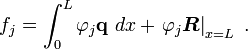
The problem with the general form of the Galerkin method is that the functions $\varphi_i$ are difficult to determine for complex domains.

This article is issued from Wikiversity - version of the Friday, April 18, 2008. The text is available under the Creative Commons Attribution/Share Alike but additional terms may apply for the media files.