Introduction to differentiation

Resources

Prelude

Arithmetic is about what you can do with numbers. Algebra is about what you can do with variables. Calculus is about what you can do with functions. Just as in arithmetic there are things you can do to a number to give another number, such as square it or add it to another number, in calculus there are two basic operations that given a function yield new and intimately related functions. The first of these operations is called differentiation, and the new function is called the derivative of the original function.

This set of notes deals with the fundamentals of differentiation. For information about the second functional operator of calculus, visit Integration by Substitution after completing this unit.

Before we dive in, we will warm up with an excursion into the mathematical workings of interest in banking.

Compound Interest

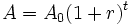
Let us suppose that we deposit an amount $A_0$ in the bank on New Year's Day, and furthermore that every year on the year the amount is augmented by a rate $r$ times the present amount. Then the amount $A$ in the bank on any given New Year's Day, $t$ years after the first is given by the expression

A=A_0(1+r)^t\,\!

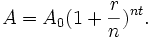
Unfortunately, if we withdraw the money three days before the New Year, we don't get any of the interest payment for that year. A fairer system would involve calculating interest $n$ times a year at the rate $r/n$ . In fact this gives us a slightly different value even if we take our money out on a New Year's Day, because every time we calculate interest, we receive interest on our previous interest. The amount $A$ we receive with this improved system is given by the expression

A=A_0(1+\frac{r}{n})^{nt}.

With this flexible system, we could set $n$ to $12$ to compound every month, or to $365$ to compound every day or to about $31536000$ to compound every second. But why stop there? Why not compound the interest every moment? What is really meant by that is this: as we increase $n$ does the value for $A$ get ever greater with $n$ or does it approach some reasonable quantity? If the latter is the case, then it is meaningful to ask, "What does $A$ approach?" As we can see from the following table with sample values, this is in fact the case.

$A_0=1$ , $r=.025$ , $t=1$
$n$	$A$
1	1.02500
12	1.02529
365	1.02531
31536000	1.02532
100000000	1.02532

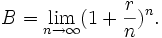
As we can see, as $n$ goes off toward infinity, $A$ approaches a finite value. Taking this to heart, we may come to our final system in which we define $A$ as follows:

A=\lim_{n\rightarrow \infty}A_0(1+\frac{r}{n})^{nt}.

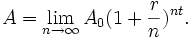
Thus we set $A$ now not t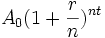o $A_0(1+\frac{r}{n})^{nt}$ evaluated for some large $n$ , but rather to the limit of that value as $n$ approaches infinity. This is the formula for continually compounded interest. To clean up this formula, note that neither $A_0$ nor $t$ "interfere" in any way with the evaluation of the limit, and may consequently be moved outside of the limit without affecting the value of the expression:

A=A_0B^t\,\!

where

B=\lim_{n\rightarrow \infty}(1+\frac{r}{n})^n.

We can see from the form of the expression that $A$ increases exponentially with $t$ much as it did in our very first equation. The difference is that the original base $(1+r)$ has been replaced with the base $B$ which we have yet to simplify.

Take a moment to step back and do the following exercises:

Without looking back, see if you can write down the expressions that represent
- yearly interest
- semiannual interest
- monthly interest
- interest $n$ times a year
- continually compounded interest
Think about how much money you have. Figure out how long you would have to leave your money in a bank that compounds interest monthly before you became a millionaire, with a yearly interest rate of
- .02 (common for a savings account)
- .07 (average gain in the US stock market over a reasonably long period).

Finding the Base

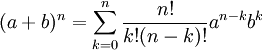
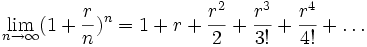
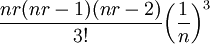
In order to shed some light on the expression whose value we call $B$ , we shall make use of the following expansion, known as the Binomial Theorem:

(a + b)^n = a^n + na^{n-1}b + \frac{n(n-1)}{2}a^{n-2}b^2 + \dots + \frac{n(n-1)(n-2)\dots(n-(k-1))}{k!}a^{n-k}b^k + \dots + nab^{n-1} + b^n.

By applying it to our limit, we get

B=\lim_{n\rightarrow \infty}(1+\frac{r}{n})^n = \lim_{n\rightarrow \infty}(1+n(\frac{r}{n})+\frac{n(n-1)}{2}(\frac{r}{n})^2 +\frac{n(n-1)(n-2)}{3!}(\frac{r}{n})^3 + \dots) =1+r+\frac{r^2}{2}+\frac{r^3}{3!}+\frac{r^4}{4!}+\dots

This last step may seem mystifying at first. What happened to the limit? And where did all of the $n$ 's go? In fact it was the evaluation of the limit that allowed us to remove the $n$ 's. More exactly, as 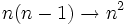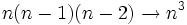$n\rightarrow\infty$ , so too $n(n-1)\rightarrow n^2$ , $n(n-1)(n-2)\rightarrow n^3$ , etc., so that the top left and bottom right of each term cancel to produce the last expression.

Take a moment to look over the following exercises. Take the time to follow the trains of thought that are newest to you.

The Pascal triangle, one of the world's most famous number patterns, popularized by the Seventeenth-Century mathematician Blaise Pascal, is shown on the right. What does this have to do with the Binomial Theorem?
The factorial (!) may seem like a silly operation to have its own name, but as it turns out it is one of the most common operations in both statistics and pure math.
- What is $100!/98!$ ?
- Which is bigger $1000!$ or $2^{1000}$ ?
The Binomial Theorem is sometimes stated $(a+b)^n=\sum_{k=0}^n\frac{n!}{k!(n-k)!}a^{n-k}b^k$ . Is this the same as the formula we used?
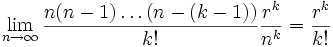In the proof, we made use of the fact that . Does this make sense based on what you know about limits?
- What is $\lim_{x\rightarrow\infty}\frac{x^5+x^4+x^3+x^2+x+1}{x^5}$ ?
Without looking back, can you remember how it is that we used binomial expansion to show that $\lim_{n\rightarrow \infty}(1+\frac{r}{n})^n = 1+r+\frac{r^2}{2}+\frac{r^3}{3!}+\frac{r^4}{4!}+\dots$ ?

						1
					1		1
				1		2		1
			1		3		3		1
		1		4		6		4		1
	1		5		10		10		5		1
1		6		15		20		15		6		1

The Birth of $e$

Now comes a real surprise. As it turns out, the infinite polynomial above is in fact exponential in 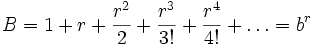$r$ . That is, $B = 1+r+\frac{r^2}{2}+\frac{r^3}{3!}+\frac{r^4}{4!}+\dots = b^r$ , for some $b$ . In order to show this far-from-obvious fact, I offer the following.

1+r+\frac{r^2}{2}+\frac{r^3}{3!}+\frac{r^4}{4!}+\dots = \lim_{n\rightarrow \infty}\bigg(1+nr\bigg(\frac{1}{n}\bigg)+\frac{nr(nr-1)}{2}\bigg(\frac{1}{n}\bigg)^2 +\frac{nr(nr-1)(nr-2)}{3!}\bigg(\frac{1}{n}\bigg)^3 + \dots \bigg)

= \lim_{n\rightarrow\infty}\bigg(1+\frac{1}{n}\bigg)^{nr} = \Bigg(\lim_{n\rightarrow\infty}\bigg(1+\frac{1}{n}\bigg)^n\Bigg)^r = \bigg(1+1+\frac{1}{2}+\frac{1}{3!}+\frac{1}{4!}+\dots \bigg)^r

To this last infinite series of numbers, define the quantity to be $e$ :

e=1+1+\frac{1}{2}+\frac{1}{3!}+\frac{1}{4!}+\dots

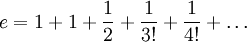$e$ , an irrational (and in fact transcendental) number, has the approximate value 2.71828, which you may easily verify on a standard pocket or graphing calculator.

There are a few things to think about.

The first line in the preceding derivation was motivated by my knowledge of the outcome.
1. Convince yourself that the two expressions are in fact equal to one another.
  - Evaluate the term $\frac{nr(nr-1)(nr-2)}{3!}\bigg(\frac{1}{n}\bigg)^3$ for $r=.02$ and $n=10000$ . How does that compare to $\frac{r^3}{3!}$ ? How about with $n=10000000$ ?
2. Now that you have convinced yourself that I may do it, ask yourself why I would do it.
  - Using the reverse Binomial Theorem, do you understand how it leads to the next expression?
Is the equation $1+r+\frac{r^2}{2}+\frac{r^3}{3!}+\frac{r^4}{4!}+\dots = \bigg(1+1+\frac{1}{2}+\frac{1}{3!}+\frac{1}{4!}+\dots\bigg)^r$ something that one would predict merely from the rules of exponents or distribution?
What makes certain seemingly uninteresting numbers so profoundly central to mathematics, such as $0$ , $1$ , $\pi$ , and $e$ ?

Back to the Start

From here, everything cascades back to our original goal, namely to find a usable formula for continually compounded interest. $B = e^r \rightarrow A=A_0(e^r)^t \rightarrow A=A_0e^{rt}$ . And there she is.

Take a moment to do the following exercises.

Think about how much money you have. How long will it take to become millionaire if you leave the money in a bank with yearly interest of .025
- that compounds interest yearly?
- that compounds interest continually?
Seeing as the values with and without continually compounded interest are very close to one another, what does that tell you about the two equations used?
- Both formulas are of the form $A=A_0($ _____ $)^t$ . Compare the various values that we have put in this blank, especially the in the equations for yearly and continually compounded interest.
- How close in value is $(1+r)$ to $e^r$ ? Does that surprise you?
- Now look at the infinite series version of the function $e^r$ . Does it still surprise you that $(1+r)$ and $e^r$ are so close in value?

Commentary

The formula itself, however, is quite forgettable. In fact, as you may have guessed, the importance of compounded interest pales in comparison to the importance of the ideas we stumbled upon on the way, namely limits and $e$ . It is these two things that beg for us to go further into the heart of the life and being of functions. That wish is called calculus. And it all starts rather innocently with the derivative…

Notion of secant, slope,

The slope of a curve is most usefully approached by considering the simplest curve, the straight line. So, imagine a line plotted on square graph paper, of the kind familiar to just about every schoolchild. What can you say about such a line? We suppose for our discussion here that the line goes off your sheet of paper on both sides, and keeps going forever. Take your page and look at it. A line might be flat, that is parallel to the bottom of the page. It might be vertical, parallel to the sides of the page, or it might lie between these two extremes, not as flat as the first, and not as steep as the second.

The first part of the idea of 'slope' is that of steepness. How steep is the line, taking the horizontal line and a vertical line as our two extremes?

Our flat horizontal line has a slope of zero - nothing happens to the y's whatever you do to the x's, think of cycling in parts of the Netherlands for example.

A line at 45 degrees to the horizontal (that is exactly half way between vertical (90 degrees) and horizontal (0 degrees) has a slope of 1 (this would be a brutal to impossible hill for a bicycle, and very tough on foot). As it goes across one unit, it also goes up (or down) one unit.

Our vertical line is more interesting, if harder to cycle on. The slope is not defined, and as our line gets closer and closer to vertical, the slope gets bigger and bigger without limit.

The second part of the idea of slope captures something slightly different. It captures the idea of direction. Look at your line again. As it goes to your right does it go up the page, or down the page? If it was a road going up a hill would it be hard to follow it on a bicycle(going up), or very easy (going down)? This is expressed in the slope of a line by saying that a line has a positive slope if, as it goes across, it also goes up, (or as the y's increase the x's increase too). A line is said to have a negative slope if it goes down as it goes across, (or as the y's increase the x's decrease). As a cyclist you want a negative slope, unless you're in training.

The Derivative

Definition

Given a function $y = f(x)$ , we define the derivative $f'(x)$ to be

f'(x)=\lim_{h\rightarrow 0}{\frac{f(x+h)-f(x)}{h}}

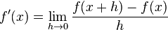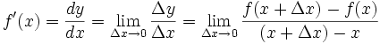
This definition is motivated by the proportion 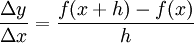$\frac{\Delta y}{\Delta x}=\frac{f(x+h)-f(x)}{h}$ , which for any h defines the slope of a line, when f is linear. Because of the nature of the calculation, the derivative can be figuratively thought of as the ratio between an infinitesimal dy and an infinitesimal dx and is often written $\frac{dy}{dx}$ . Both functional notation $\left ( f'(x) \right )$ and infinitesimal or Leibniz notation $\left ( \frac{dy}{dx} \right )$ have their virtues. In operator theory, the derivative of a function $f$ is sometimes written as $D_x f \,\!$ .

Using the definition above, what is ?
- Note that this is a short way of asking, if $f(x)=x^2$ , what is $f'(x)$ ? One may also ask, what is $[x^2]'$ ?
If you have trouble remembering the definition of the derivative, it's much more important to know what it means, that is, why it's defined how it is. Remember it like this:
- $f'(x)=\frac{dy}{dx}=\lim_{\Delta x\rightarrow 0}\frac{\Delta y}{\Delta x}=\lim_{\Delta x\rightarrow 0}\frac{f(x+\Delta x)-f(x)}{(x+\Delta x) - x}$ .
- From this we get the definition as stated above, $f'(x)=\lim_{h\rightarrow 0}{\frac{f(x+h)-f(x)}{h}}$ .
What kinds of functions have derivatives? What would a function need to have, for it not to have a derivative at some point?

Properties

The derivative satisfies a number of fundamental properties

Linearity

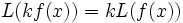An operator $L$ is called linear if $L(f(x)+g(x))=L(f(x)) +L(g(x))$ and $L(kf(x))=kL(f(x))$ for any constant $k$ . To show that differentiation is a linear operator, we must show that $[f(x)+g(x)]'=f'(x)+g'(x)$ and $[kf(x)]'=kf'(x)$ for any constant $k$ .

[f(x)+g(x)]'=\lim_{h\rightarrow 0}\frac{(f(x+h)+g(x+h))-(f(x)+g(x))}{h}

=\lim_{h\rightarrow 0}(\frac{f(x+h)-f(x)}{h}+\frac{g(x+h)-g(x)}{h})=\lim_{h\rightarrow 0}\frac{f(x+h)-f(x)}{h} + \lim_{h\rightarrow 0}\frac{g(x+h)-g(x)}{h}=f'(x)+g'(x)

In other words, the differential operator (e.g., $\frac{d}{dx}$ ) distributes over addition.

[kf(x)]'=\lim_{h\rightarrow 0}\frac{kf(x+h)-kf(x)}{h}=k\lim_{h\rightarrow 0}\frac{f(x+h)-f(x)}{h}=kf'(x)

In other words, addition before and after doing differentiation are equivalent.

Fundamental Rules of Differentiation

Along with linearity, which is so simple that one hardly thinks of it as a rule, the following are essential to finding the derivative of arbitrary functions.

The Product Rule

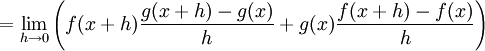
It may be shown that for functions f and g, $[f(x)g(x)]'=f(x)g'(x) + f'(x)g(x)$ . Like the other two rules, this one is not a new axiom: it is directly provable from the definition of the derivative.

$[f(x)g(x)]' = \lim_{h\rightarrow 0} \frac{f(x+h)g(x+h) - f(x)g(x)}{h} = \lim_{h\rightarrow 0} \frac{f(x+h)g(x+h) - f(x+h)g(x) + f(x+h)g(x) - f(x)g(x)}{h}$

$= \lim_{h\rightarrow 0} \left( f(x+h)\frac{g(x+h)-g(x)}{h} + g(x)\frac{f(x+h)-f(x)}{h} \right)$

$= f(x)\left( \lim_{h\rightarrow 0}\frac{g(x+h)-g(x)}{h} \right) + g(x) \left( \lim_{h\rightarrow 0} \frac{f(x+h)-f(x)}{h} \right) = f(x)g'(x) + g(x)f'(x)$ .

Chain Rule

If a function f(x) can be written as a compound function f(g(x)), one can obtain its derivative using the chain rule. The chain rule states that the derivative of f(x) will equal the derivative of f(g) with respect to g, multiplied by the derivative of g(x) with respect to x. In mathematical terms: $[ \, f(g(x)) \, ]'=f'(g(x))g'(x).$ This is commonly written as $\textstyle \frac{df}{dx} = \frac{df}{dg}\frac{dg}{dx}$ , or more explicitly $\tfrac{d}{dx}f(x) = \tfrac{d}{dg}f(g(x)) \, \tfrac{d}{dx} g(x).$

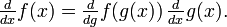
The proof makes use of an alternate but patently equivalent definition of the derivative: 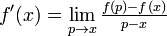$f'(x) = \lim_{p\rightarrow x}\tfrac{f(p)-f(x)}{p-x}$ . The first step is to write the derivative of the compound function in this form; one then manipulates it and obtains the chain rule.

$\begin{align} \left[f(g(x))\right]' & = \lim_{p\rightarrow x}\frac{f(g(p))-f(g(x))}{p-x} \\ & = \lim_{p\rightarrow x} \frac{f(g(p))-f(g(x))}{g(p)-g(x)} \; \frac{g(p)-g(x)}{p-x} \\ & = \lim_{g(p)\rightarrow g(x)} \frac{f(g(p))-f(g(x))}{g(p)-g(x)} \; \lim_{p\rightarrow x} \frac{g(p)-g(x)}{p-x} \\ & = f'(g(x)) g'(x). \end{align}$

In the third step, the first limit changes from p→x to g(p)→g(x). This is valid because if g is continuous at x, which it must be to have a derivative at x, then of course as p approaches x the value of g(p) approaches that of g(x).

Differentiating a nested function occurs very frequently, which makes this rule very useful.

The Power Rule

We may now readily show the relation 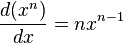$\frac{d(x^n)}{dx} = n x^{n-1}$ as follows:

$\frac{d(x^n)}{dx} = \lim_{h\rightarrow 0}\frac{(x+h)^{n}-x^n}{h} = \lim_{h\rightarrow 0}\frac{(x^n+nx^{n-1}h+\frac{n(n-1)}{2}x^{n-2}h^2+\cdots)-x^n}{h}$

$= \lim_{h\rightarrow 0}(nx^{n-1}+\frac{n(n-1)}{2}x^{n-2}h+\cdots)=nx^{n-1}+0=nx^{n-1}.$

While this derivation assumes that $n$ is an positive integer, it turns out that the same rule holds for all real $n$ . For example, $\frac{d}{dx}[\frac{1}{x}]=\frac{d(x^{-1})}{dx}=(-1)x^{-2}=-\frac{1}{x^2}$ .

Take a moment to do the following exercises.

Using the rule and linearity, find the derivatives of the following:
1. $x^{14} + 8$
2. $3x^2+x^5$
3. $\frac{1}{\sqrt{x}}$
What functions have the following derivatives?
1. $3x^2$
2. $15x^{14} + 2x$
3. $x^2$

Exponentials and logarithms

Exponentials and logarithms involve a special number denoted e.

Differentiating $e^x$

Now, recall that

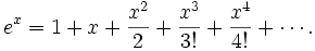
$e^x = 1 + x + \frac{x^2}{2} + \frac{x^3}{3!} + \frac{x^4}{4!} + \cdots.$

Using the three basic rules established above we can differentiate any polynomial, even one of infinite degree:

$\frac{d}{dx}e^x = 0 + 1 + \frac{2x}{2} + \frac{3x^2}{3!} + \frac{4x^3}{4!} + \cdots = 1 + x + \frac{x^2}{2} + \frac{x^3}{3!} + \cdots = e^x.$

$e^x$ is the remarkable function that is its own derivative. In other words, $e^x$ is an eigenfunction of the differential operator. Which means that the application of the differential operator on $e^x$ has the same effect as multiplication by a real number. For example, these concepts are useful in quantum mechanics.

Differentiating $\ln(x)$

The natural logarithm is the function such that if $e^y=x$ then $y=\ln(x)$ ; in other words, it is the inverse function of $e^x$ . We will make use of the chain rule (marked by the brace) in order to find its derivative:

$y=\ln(x) \rightarrow x=e^y \rightarrow \frac{dx}{dx}=\frac{d(e^y)}{dx} \rightarrow 1=\underbrace{\frac{d(e^y)}{dy}\frac{dy}{dx}}=e^y\frac{dy}{dx}=e^{\ln(x)}\frac{dy}{dx}=x\frac{dy}{dx} \rightarrow \frac{1}{x}=\frac{dy}{dx}=\frac{d(\ln(x))}{dx}.$

This conclusion, that the derivative of $\ln(x)$ is $\frac{1}{x}$ , is remarkable: it ties together two seemingly unrelated functions. Be careful, this derivative has definite values only when x > 0! (Examine the $ln(x)$ to understand why.)

Differentiating functions which are not immediately related to base $e$

Exponentials

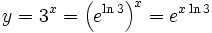
Supppose we have the function

y = 3^x \,\!

To differentiate this, we rewrite this as

y = 3^x = \left ( e^{\ln 3} \right )^x = e^{x \ln 3}

Since $\ln 3$ is a constant,

\frac{dy}{dx} = e^{x \ln 3} \cdot \ln 3 = 3^x \ln 3.

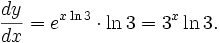
In other words, for a constant a, we have

\frac{dy}{dx} = a^x \ln a

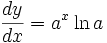whenever

y = a^x \,\!

This re-enforces the special place that $e$ has in calculus - it is the unique number for which the constant $\ln a$ is precisely equal to one.

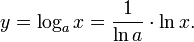
Logarithms

Let us differentiate the function

y = \log_a x\!

We already know how to differentiate $\ln x\!$ , so let's change it into another form with the base e.

y = \log_a x = \frac{1}{\ln a} \cdot \ln x.

Because $\frac {1}{\ln a}$ is a constant,

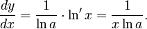
\frac{dy}{dx} = \frac{1}{\ln a} \cdot \ln' x = \frac{1}{x\ln a}.

In conclusion, for any constant a, the derivative of $\log_a x\!$ is $\frac{1}{x\ln a}$

Implicit Differentiation

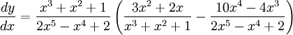
Let's suppose that

y(x) = \frac{x^3 + x^2 + 1}{2x^5 -x^4 +2}

One could find $\frac{dy}{dx}$ with the quotient rule, but for more complicated functions, it may be better to use what is called "implicit differentiation".

In this case, we take the logarithm of both sides, to obtain

\ln y = \ln \left ( \frac{x^3 + x^2 + 1}{2x^5 -x^4 +2} \right ) = \ln \left( x^3 + x^2 + 1 \right ) - \ln \left( 2x^5 -x^4 +2 \right )

or, in other words, just simply

\ln y = \ln \left( x^3 + x^2 + 1 \right ) - \ln \left( 2x^5 -x^4 +2 \right )

Differentiating the left and right hand side, we get

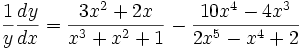
\frac{1}{y} \frac{dy}{dx} = \frac{3x^2+2x}{x^3 + x^2 + 1} - \frac{10x^4 - 4x^3}{2x^5 -x^4 +2 }

Now, multiply both sides by y, which we know is just 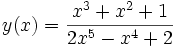$y(x) = \frac{x^3 + x^2 + 1}{2x^5 -x^4 +2}$ to obtain the answer:

{dy \over dx} = \frac{x^3 + x^2 + 1}{2x^5 -x^4 +2} \left ( \frac{3x^2+2x}{x^3 + x^2 + 1} - \frac{10x^4 - 4x^3}{2x^5 -x^4 +2 } \right )

which of course can be simplified further. You should verify that this result agrees with the quotient rule. Differentials of logarithms of functions occur frequently in places like statistical mechanics.

General exponentials and logarithms

Consider the function

y(x) = u(x)^{v(x)} = e^{v(x) \ln u(x)} \,\!

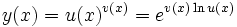
It can be immediately seen that

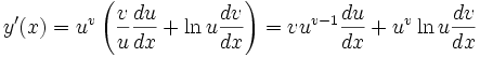
y'(x) = u^v \left ( \frac{v}{u} \frac{du}{dx} + \ln u \frac{dv}{dx} \right ) = v u^{v-1} \frac{du}{dx} + u^v \ln u \frac{dv}{dx}

Compare this result to the chain rule and power rule results. The first term results in treating v constant. The second term results in treating u constant.

Trigonometric functions

Consider the function 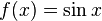$f(x) = \sin x$ . To find the derivative of $f(x)$ , we use the definition of the derivative, as well as some trigonometric identities and the linearity of the limit operator.

\lim_{h \to 0} \dfrac{f(x+h) - f(x)}{h} = \lim_{h \to 0} \dfrac{\sin(x+h) - \sin x}{h} = \lim_{h \to 0}\dfrac{\cos x\sin h + \sin x \cos h - \sin x}{h}

=\lim_{h \to 0} \cos x \dfrac{\sin h}{h} - \sin x \dfrac{1 - \cos h}{h} = \cos x\left[\lim_{h \to 0} \dfrac{\sin h}{h}\right] - \sin x \left[\lim_{h \to 0}\dfrac{1 - \cos h}{h}\right],

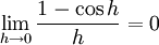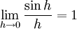and since $\lim_{h \to 0}\dfrac{1 - \cos h}{h} = 0$ and $\lim_{h \to 0} \dfrac{\sin h}{h}=1$ , the above expression simplifies to $\cos x\!$ .

Thus, the derivative of $\sin x\!$ is $\cos x\!$ .

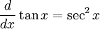
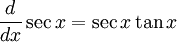
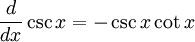
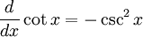
We perform the same process to find the derivatives of the other trigonometric functions (try to derive them on your own as an exercise). Since these derivatives come up quite often, it would behoove (advantageous to) you to memorize them.

$\dfrac{d}{dx}\sin x = \cos x$

$\dfrac{d}{dx}\cos x = -\sin x$

$\dfrac{d}{dx}\tan x = \sec^2 x$

$\dfrac{d}{dx}\sec x = \sec x \tan x$

$\dfrac{d}{dx}\csc x = -\csc x \cot x$

$\dfrac{d}{dx}\cot x = -\csc^2 x$

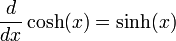
Hyperbolic functions

The rules for differentiation involving hyperbolic functions behave very much like their trigonometric counterparts. Here,

$\textrm{sinh}(x) = \frac{e^{x} - e^{-x}}{2}$

$\cosh(x) = \frac{e^{x} + e^{-x}}{2}$

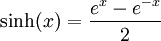
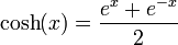
so it can be seen that

$\frac{d}{dx} \sinh(x) = \cosh(x)$

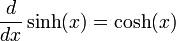
and $\frac{d}{dx} \cosh(x) = \sinh(x)$

This article is issued from Wikiversity - version of the Tuesday, January 12, 2016. The text is available under the Creative Commons Attribution/Share Alike but additional terms may apply for the media files.