Introduction to Likelihood Theory/The Basic Definitions

Formal Probability Review

Let $D$ be a set contained in $R^{k}$ , and $dm\left(x\right)$ is the counting measure if $D$ is discrete, Lebesgue measure if $D$ is continuous and Steltjes measure otherwise (if you don't know what a measure function in a $\sigma-\mathrm{algebra}$ is, lookup in w:measure (mathematics) or just consider that if $D$ is continuous the integrals below are the usual integrals from calculus, and the integrals resume to summation over $D$ for discrete sets).

Definition.: A function $f(x):D\rightarrow R$ is a probability density function (abbreviated pdf) if and only if
$\int_{-\infty}^{\infty}fdm(x)=1$
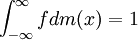
and
$f(x)\geq 0~\forall x \in R$ .
We say that a variable $X$ has pdf f if the probability of $X$ being in any set $S$ is given by the expression
$\int_{S}^{}f(x)dm$
(if you don't know measure theory, consider that $S$ is an interval on the real line).

Exercise 1.1 - Show that 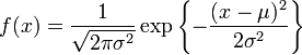$f(x)=\frac{1}{\sqrt{2\pi\sigma^{2}}}\exp\left\{-\frac{(x-\mu)^{2}}{2\sigma^{2}}\right\}$ is a pdf with $D=R$ , $\mu \in R$ and $\sigma^{2}>0$ .
Exercise 1.2 - Show that we can build a distribution function using the function $g(x)=0$ , if $x<k$ , $f(x)$ otherwise ( $k$ is any real number, $f$ is defined in the previous exercise) by multiplying it with an appropriate constant. Find the constant. Generalize it for any pdf defined on the real line.
Exercise 1.3 - If $X$ has distribuition $f$ with $\mu=1$ and $\sigma^{2}=1$ , what is the distribution of the function $Y=X^{2}$ ?(Calculate it, don't look it up on probability books). In statistics, the term probability density function is often abbreviated to density.

Definition.: Let $X$ be a random variable with density $f$ . The Cumulative Distribution Function (cdf) of $X$ is the function defined as

F(x)=\int_{-\infty}^{x}fdm(x)

This function is often called distribution function or simply distribution. Since the distribution determines uniquely the density, the terms distribution and density are used by statisticians as synonymous (provided no ambiguity arises from the context).
Exercise 1.4 - Prove that every cdf is nondecreasing.

Definition.: Let $X$ be a random variable. We call the expectation of the function $g(X)$ the value

E[g(X)]=\int_{-\infty}^{\infty}gfdm(x)

where $f$ is the density of $X$ . The expectation og the identity function is called expectation of $X$ .
Exercise 1.5 - Compute the expectation of the random variables defined in Exercise 1.1.
Exercise 1.6 - Show that $E[c]=c$ for any constant $c$ .
Exercise 1.7 - Show that $E[g(x)+c]=E[g(x)]+c$ for any constant $c$ .

In The Beginning There Were Chaos, Empirical Densities and Samples

A population is a collection of objects (collection, not a proper set or class in a Logicist point of view) where each object has an array of measurable variables. Examples include the set of all people on earth together with their heights and weights and the set of all fish in a lake together with artificial marks on them, whre this latter case is found in capture-recapture studies (I suggest you look into Wikipedia and find out what is a capture-recapture study). Let $s$ be an element of a population and $V(s)$ be the array of measurable variables mensured in the object $s$ (for an example, $s$ is a man and $V(s)$ is his height and weight measured at some arbitrary instant, or $s$ is a fish and $V(s)$ is $1$ if he has a man-made mark on it and $0$ otherwise). A sample of a population $P$ is a collection $S$ (again, not a set) where $s \in S\Rightarrow \exists r \in P$ such that $V(s)=V(r)$ .

There are two main methods for generating samples: Sampling with replacement and Sampling without replacement (duh!). In the former, you randomly select a element $a_{1}$ of $P$ , and call the set $S_{1}=\left\{a_{1}\right\}$ your first subsample. Define you (n+1)-th subsample as the set $S_{n+1}=S_{n}\bigcup \left\{R(P-S_{n})\right\}$ , where $R(X)$ is a function returning a randomly chosen element of $X$ . Any subsample you pick generated using the definitions above will be called a sample without replacement, and is the more intuitive kind of sample but also one of the most complicated to obtain in a real world situation. In the former, we have $S_{1}$ and $R(X)$ defined in the same way above, but in this case we have $S_{n+1}=S_{n}\bigcup \left\{s_{n}:V(R(P)=V(s_{n})\right\}$ . Samples with replacement have the exquisite property that they have different objects with same characteristics.

TODO.: Some stuff on empirical densities and example of real world sampling techniques.

Likelihoods, Finally

Given a random vector $Y=\left[Y_{1}~Y_{2}~\cdots~Y_{n}\right]^{T}$ with density $f_{Y}(y,\theta)$ , where $\theta$ is a vector of parameters, and an observation $y'=\left[y'_{1}~y'_{2}~\cdots~y'_{n}\right]^{T}$ of $Y$ , we define the likelihood function associated with $y'$ as

L\left(\theta\right)=f_{Y}\left(y',\theta\right)

This is a function of $\theta$ , but not of $Y$ , of an observation $y$ or any other related quantity, for $L(\theta)$ is the restriction of the function $f_{Y}$ , which is a function of $n+dim(\theta)$ , to a subspace where the $y$ are fixed.

In many applications we have that, for all $j,i \in \{0,1,\ldots,n\}$ , $Y_{j}$ and $Y_{i}$ are independent. Suppose that we draw a student from a closed classroom at random, record his height $y_{1}$ , and put him back. If we repeat the proccess $n$ times, the set of heights measured forms an observed vector $y'=\left[y'_{1}~y'_{2}~\cdots~y'_{n}\right]^{T}$ , and our $Y$ variable is the distribution of the height of the students in that classroom. Then we have our independence supposition fullfilled, as it will be for any sampling scheme with replacement. In the case where the supposition is true, the above definition of likelihood finction is equivalent to

L(\theta)=\prod_{j=1}^{n}f_{Y_{j}}(y',\theta)

where $f_{Y_{j}}(y',\theta)$ is the probability density function of the variable $Y_{j}$ .
Exercise 3.1: Let $X_{j}$ have a Gaussian density with zero mean and unit variance for all $j$ . Compute the likelihood function of $Y_{1}=X_{1}$ and $Y_{2}=X_{1}+X_{2}$ for an arbitrary sample.

Intuitive Meaning?

This function we call likelihood is not directly related to the probability of events involving $Y$ or any proper subset of it, despite its name, but it has a non-obvious relation to the probability of the sample as a whole being selected in the space of all the possible samples. This can be seen if we use discrete densities (or probability generating functions). Supose that each $y_{j}$ has a binomial distribution with $m$ tries and succes probability $p_{j}$ , and they are independent. So the likelihood function associated with a sample $y'=\left[y'_{1}~y'_{2}~\cdots~y'_{n}\right]^{T}$ is

L(\theta)=\prod_{j=1}^{n}C_{m,y'_{j}}p^{y'_{j}}(1-p)^{1-y'_{j}}

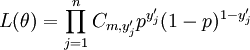
where each $y'_{j}$ is in $\{0,1\}$ , and $C_{m,k}$ means $choose\left(m,k\right)$ . This function is the probability of this particular sample appear considering all the possible samples of the same size, but this trail of thought only works in discrete cases with finite sample space.
Exercise 4.1: In the Binomial case, does $L(\theta_{1})>L(\theta_{0})$ has any probabilistic meaning? If the observed values are throws of regular fair coins, what can you expect of the function $L(\theta)$ ?

But the likelihood has a comparative meaning. Supose that we are given two observations of $Y$ , namely $Y_{1}$ and $Y_{2}$ . Then each observation defines a likelihood function, and for each fixed $\theta_{0}$ , we may compare their likelihoods $L_{1}\left(\theta_{0}\right)$ and $L_{2}\left(\theta_{0}\right)$ to argue that the one with bigger value occurs more likely. This argument equivalent to Fisher's rant against Inverse Probabilities.

Bayesian Generalization

Even if most classical statisticians (also called "frequentists") complain, we must talk about this generalization of the likelihood function concept. Given that the vector $Y$ has a density conditional on $X$ called $f_{Y|X}(y|x)$ and that we have a observation $x'$ of $X$ (I said $X$ , forget about observations of $Y$ in this section!), we will play a little with the function

L\left(Y\right)=f_{Y|X}\left(y|x'\right)

Before anything, Exercise 5.1: Find two tractable discrete densities with known conditional density and compute their likelihood function. Relate $L\left(Y\right)$ to $L\left(X\right)$ .

On to Maximum Likelihood Estimation

Thank you for reading

Some comments are needed. The "?" mark in the previous section title is proposital, to show how this might be confusing. It needs more exercises and examples from outside formal probability. The way this thing is right now needs a good background in formal probability (high level) and much more experience with sampling.

This article is issued from Wikiversity - version of the Thursday, March 27, 2014. The text is available under the Creative Commons Attribution/Share Alike but additional terms may apply for the media files.