Introduction to Elasticity/Stress example 3

Example 3

Given:

A stress field whose components in the basis $(\mathbf{e}_1, \mathbf{e}_2, \mathbf{e}_3)\,$ are given by the matrix

[\boldsymbol{\sigma}] = \begin{bmatrix} 6~x_1~x_3^2 & 0 & -2~x_3^3 \\ 0 & 1 & 2 \\ -2~x_3^3 & 2 & 3~x_1^2 \end{bmatrix}

Find:

Assuming negligible body forces, show whether this field satisfies equilibrium.
Find the traction acting at a point P whose position vector is $\mathbf{x} = 2~\mathbf{e}_1 + 3~\mathbf{e}_2 + 2~\mathbf{e}_3 \,$ acting on a plane $2~x_1 + x_2 - x_3 = 5\,$ .
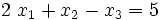Determine the normal traction at this point on the plane.
Determine the projected shear traction at this point on the plane.
Determine the principal stresses at point P.
Determine the principal directions of stress at point P.

Solution

This problem is very similar to example 2.

The stress is a function of $x_1\,$ and $x_3\,$ . We first plug the stress into the equilibrium equations (Cauchy's first law) and find that the sum is zero. Hence the stress satifies equilibrium.

Next, we find the stress at the given point byplugging in the values of $x_1\,$ and $x_3\,$ into the given stress.

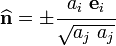
Then we find the normal to the given plane $a_i~x_i = b\,$ using the relation

\widehat{\mathbf{n}} = \pm \cfrac{a_i~\mathbf{e}_i}{\sqrt{a_j~a_j}}

and find the traction vector and thenormal and projected shear tractions.

We find the eigenvalues (principal stresses) by first forming the cubic characteristic equation and then solving for it. Then we plug the values of the principal stresses into the eigenfunction and solve for the direction of the principal strains.

Since the stress tensor is symmetric, we need an extra relation between $n_1\,$ , $n_2\,$ , and $n_3\,$ to reduce the system down to two equations and two unknowns. This relation is 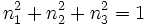$n_1^2 + n_2^2 + n_3^2 = 1\,$ , which means that each eigenvector is a unit vector.

The Maple output is shown below.


> with(linalg):
> sigma :=
> linalg[matrix](3,3,[6*x1*x3^2,0,-2*x3^3,0,1,2,-2*x3^3,2,3*x1^2]);

                           [       2              3]
                           [6 x1 x3     0    -2 x3 ]
                           [                       ]
                  sigma := [   0        1      2   ]
                           [                       ]
                           [      3              2 ]
                           [ -2 x3      2    3 x1  ]

> e1 := linalg[matrix](3,1,[1,0,0]):
> e2 := linalg[matrix](3,1,[0,1,0]):
> e3 := linalg[matrix](3,1,[0,0,1]):
> sigi1i := diff(sigma[1,1],x1)+diff(sigma[2,1],x2)+diff(sigma[3,1],x3);

                             sigi1i := 0

> sigi2i := diff(sigma[1,2],x1)+diff(sigma[2,2],x2)+diff(sigma[3,2],x3);

                             sigi2i := 0

> sigi3i := diff(sigma[1,3],x1)+diff(sigma[2,3],x2)+diff(sigma[3,3],x3);

                             sigi3i := 0

> X := evalm(2*e1 + 3*e2 + 2*e3):
> sig := linalg[matrix](3,3):
> for i from 1 to 3 do
>  for j from 1 to 3 do
>   sig[i,j] := eval(eval(eval(sigma[i,j], x1 = X[1,1]), x2 =X[2,1]), x3
> = X[3,1]);
>  end do;
> end do;
> evalm(sig);

                          [ 48    0    -16]
                          [               ]
                          [  0    1      2]
                          [               ]
                          [-16    2     12]

> a1 := 2: a2 := 1: a3 := -1: ajaj := sqrt(a1*a1 + a2*a2 + a3*a3):
> n := evalm(a1*e1/ajaj + a2*e2/ajaj + a3*e3/ajaj);

                                 [  1/2 ]
                                 [ 6    ]
                                 [ ---- ]
                                 [  3   ]
                                 [      ]
                                 [  1/2 ]
                            n := [ 6    ]
                                 [ ---- ]
                                 [  6   ]
                                 [      ]
                                 [   1/2]
                                 [  6   ]
                                 [- ----]
                                 [   6  ]

> sigT := transpose(sig):
> t := evalm(sigT&*n);

                                 [    1/2]
                                 [56 6   ]
                                 [-------]
                                 [   3   ]
                                 [       ]
                            t := [   1/2 ]
                                 [  6    ]
                                 [- ---- ]
                                 [   6   ]
                                 [       ]
                                 [    1/2]
                                 [-7 6   ]

> tT := transpose(t):
> N := evalm(tT&*n): Nt := evalf(N[1,1]);

                          Nt := 44.16666667

> tdott := evalm(tT&*t):
> St := evalf(sqrt(tdott[1,1] - N[1,1]^2));

                          St := 20.83599984

> I1 := sig[1,1]+sig[2,2]+sig[3,3];

                               I1 := 61

> I2 := sig[1,1]*sig[2,2] + sig[2,2]*sig[3,3] + sig[3,3]*sig[1,1] -
> sig[1,2]*sig[2,1] - sig[2,3]*sig[3,2] - sig[3,1]*sig[1,3];

                              I2 := 376

> I3 := det(sig);

                              I3 := 128

> prinSig := solve(x^3 - I1*x^2 + I2*x - I3 = 0, x):
> s1 := evalf(prinSig[1]); s2 := evalf(prinSig[2]); s3 :=
> evalf(prinSig[3]);

                                              -8
                    s1 := 54.09271724 - 0.2 10   I


                                                  -8
               s2 := 0.361501126 - 0.8160254040 10   I


                                                  -8
               s3 := 6.545781610 + 0.9160254040 10   I

> sig1 := 54.09271724; sig2 := 6.545781610; sig3 := .361501126;

                         sig1 := 54.09271724


                         sig2 := 6.545781610


                         sig3 := 0.361501126

> with(LinearAlgebra): Id := IdentityMatrix(3):
> Left1 := evalm(sig - sig1*Id):
> n3 := sqrt(1 - n1^2 - n2^2):
> n := linalg[matrix](3,1,[n1,n2,n3]):
> Ax1 := evalm(Left1 &* n):
> sols1 := solve({Ax1[1,1] = 0, Ax1[2,1] = 0});

          sols1 := {n2 = 0.01340427809, n1 = -0.9344527487}

> N1_1 := sols1[2]; N1_2 := sols1[1]; N1_3 := sqrt(1 -
> (.1340427809e-1)^2 - (-.9344527487)^2);
> 

                      N1_1 := n1 = -0.9344527487


                      N1_2 := n2 = 0.01340427809


                         N1_3 := 0.3558347730

> Left2 := evalm(sig - sig2*Id):
> Ax2 := evalm(Left2 &* n):
> sols2 := solve({Ax2[1,1] = 0, Ax2[2,1] = 0});

           sols2 := {n1 = 0.3412802400, n2 = 0.3188798847}

> N2_1 := sols2[1]; N2_2 := sols1[2]; N2_3 := sqrt(1 - (.3412802400)^2 -
> (.3188798847)^2);

                      N2_1 := n1 = 0.3412802400


                      N2_2 := n1 = -0.9344527487


                         N2_3 := 0.8842191001

> Left3 := evalm(sig - sig3*Id):
> Ax3 := evalm(Left3 &* n):
> sols3 := solve({Ax3[1,1] = 0, Ax3[2,1] = 0});

           sols3 := {n1 = 0.1016162335, n2 = -0.9477003447}

> N3_1 := sols3[1]; N3_2 := sols3[2]; N3_3 := sqrt(1 - (.1016162335)^2 -
> (-.9477003447)^2);

                      N3_1 := n1 = 0.1016162335


                      N3_2 := n2 = -0.9477003447


                         N3_3 := 0.3025528017

This article is issued from Wikiversity - version of the Monday, February 01, 2016. The text is available under the Creative Commons Attribution/Share Alike but additional terms may apply for the media files.