Introduction to Elasticity/Stress example 2

< Introduction to Elasticity

Example 2

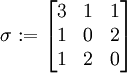
Given: A homogeneous stress field with components in the basis $(\mathbf{e}_1, \mathbf{e}_2, \mathbf{e}_3)\,$ given by

\left[\boldsymbol{\sigma}\right] = \begin{bmatrix} 3 & 1 & 1 \\ 1 & 0 & 2 \\ 1 & 2 & 0 \end{bmatrix} \text{(MPa)}

Find:

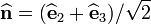The traction ( $\mathbf{t}\,$ ) acting on a surface with unit normal $\widehat{\mathbf{n}} = (\widehat{\mathbf{e}}_2+\widehat{\mathbf{e}}_3)/\sqrt{2}$ .
The normal traction ( $\mathbf{t}_n\,$ ) acting on a surface with unit normal $\widehat{\mathbf{n}} = (\widehat{\mathbf{e}}_2+\widehat{\mathbf{e}}_3)/\sqrt{2}$ .
The projected shear traction ( $\mathbf{t}_s$ ) acting on a surface with unit normal $\widehat{\mathbf{n}} = (\widehat{\mathbf{e}}_2+\widehat{\mathbf{e}}_3)/\sqrt{2}$ .
The principal stresses.
The principal directions of stress.

Solution

Here's how you can solve this problem using Maple.
with(linalg):

sigma := linalg[matrix](3,3,[3,1,1,1,0,2,1,2,0]);

\sigma := \begin{bmatrix} 3 & 1 & 1 \\ 1 & 0 & 2 \\ 1 & 2 & 0 \end{bmatrix}

e2 := linalg[matrix](3,1,[0,1,0]);

\mathit{e2} := \begin{bmatrix} 0 \\ 1 \\ 0 \end{bmatrix}

e3 := linalg[matrix](3,1,[0,0,1]);

\mathit{e3} := \begin{bmatrix} 0 \\ 0 \\ 1 \end{bmatrix}

n := evalm((e2+e3)/sqrt(2));

n := \begin{bmatrix} 0 \\ { \frac {\sqrt{2}}{2}} \\ [2ex] { \frac {\sqrt{2}}{2}} \end{bmatrix}

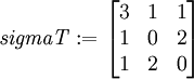
sigmaT := transpose(sigma);

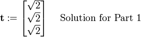
\mathit{sigmaT} := \begin{bmatrix} 3 & 1 & 1 \\ 1 & 0 & 2 \\ 1 & 2 & 0 \end{bmatrix}

t := evalm(sigmaT&*n);

\mathbf{t} := \begin{bmatrix} \sqrt{2} \\ \sqrt{2} \\ \sqrt{2} \end{bmatrix} ~~~~ \text{Solution for Part 1}

tT := transpose(t);

\mathit{tT} := \begin{bmatrix} \sqrt{2} & \sqrt{2} & \sqrt{2} \end{bmatrix}

N := evalm(tT&*n);

N := \begin{bmatrix} 2 \end{bmatrix} ~~~~ \text{Solution for Part 2}

tdott := evalm(tT&*t);

\mathit{tdott} := \begin{bmatrix} 6 \end{bmatrix}

S := sqrt(tdott[1,1] - N[1,1]^2);

S := \sqrt{2} ~~~~ \text{Solution for Part 3}

sigPrin := eigenvals(sigma);

\mathit{sigPrin} := 1, \,-2, \,4 ~~~~ \text{Solution for Part 4}

dirPrin := eigenvects(sigma);

\mathit{dirPrin} := [1, \,1, \,\{[-1, \,1, \,1]\}], \,[-2, \,1, \,\{[0, \,-1, \,1]\}], \,[4, \,1, \,\{[2, \,1, \,1]\}]

dirPrin[1];

[1, \,1, \,\{[-1, \,1, \,1]\}] ~~~~ \text{Solution for Part 5}

dirPrin[2];

[-2, \,1, \,\{[0, \,-1, \,1]\}] ~~~~ \text{Solution for Part 5}

dirPrin[3];

[4, \,1, \,\{[2, \,1, \,1]\}] ~~~~ \text{Solution for Part 5}

This article is issued from Wikiversity - version of the Monday, February 01, 2016. The text is available under the Creative Commons Attribution/Share Alike but additional terms may apply for the media files.