Introduction to Elasticity/Polynomial solutions
< Introduction to ElasticityUsing the Airy Stress Function : Polynomial Solutions
|
Given: 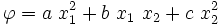 Find the problem which fits this solution.  This is a homogeneous stress field. An infinite number of problems can satisfy these conditions. |
|
Given:  Find the problem which fits this solution.  An infinite set of problems can have this stress field as a solution. If  which corresponds to a plane stress beam under pure bending.
| ||
 , then
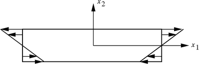
|
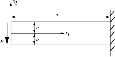
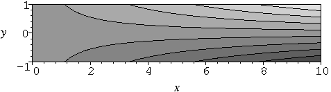
Consider a cantilevered beam that is fixed at one end and has a vertical force F applied at the free end.
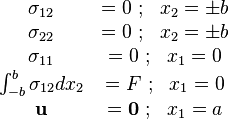
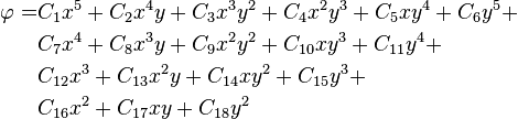
The boundary conditions on the beam are We will use Maple to solve the problem. First, assume a polynomial Airy stress function that has a high enough order. In this case a fourth order polynomial will suffice
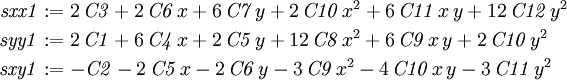
Take the derivatives of the stress function to obtain the expressions for the stresses.
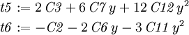
Next, use the command We now find the tractions on and on On The stress function is order 4, so the stresses are order 2 in x and y. The tractions on We calculate the coefficients of each power of x in these expressions as
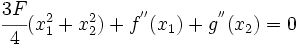
The biharmonic equation is 4th order, so applying it to a 4th order polynomial
generates a constant. And this constant must be equal to zero.
We also calculate the three force resultants on x=0 by integrating over y:
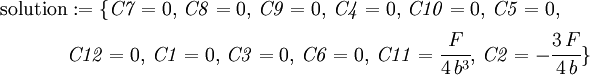
We now solve for the constants so as to satisfy (i) the strong boundary
conditions, (ii) the biharmonic equation and (iii) the weak boundary
conditions.
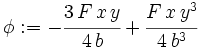
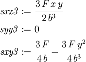
Notice that there are more equations than there are constants. Some of the equations are not linearly independent. However, Maple can handle this if there is a solution. Substitute the solution into the original stress function and calculate the final stresses.
and
Displacement Boundary Condition The displacement potential function must satisfy the relations
In this problem, 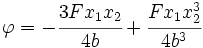 Therefore,  Integrating, 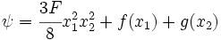
 which means that 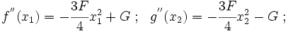 These can be integrated to find The displacements are given by ![\begin{matrix}
u_1 &= -\cfrac{P}{2EI}(a^2-x_1^2)x_2 -\cfrac{P(2+\nu)}{6EI}x_2^3
+\cfrac{P(1+\nu)b^2}{8EI}x_2\\
u_2 &= -\cfrac{Pa^3}{6EI}\left[2
-\cfrac{3x_1}{a}\left(1-\cfrac{\nu x_2^2}{a^2}\right)
+ \cfrac{x_1^3}{a^3} +
\cfrac{3b^2(1+\nu)}{4a^2}\left(1-\cfrac{x_1}{a}\right)\right]
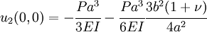
\end{matrix}](../I/m/c6131c40b0d92fe02a6cfce9d3c2a229.png) where
![u_2(x_1,0) = -\cfrac{Pa^3}{6EI}\left[2 -\cfrac{3x_1}{a} + \cfrac{x_1^3}{a^3} + \cfrac{3b^2(1+\nu)}{4a^2}\left(1-\cfrac{x_1}{a}\right)\right]](../I/m/e463618ee7461454824ffb8221deaf3c.png)
 | |||

 .
.


 , we have
 or
or  might therefore be polynomials in
  of order 2.
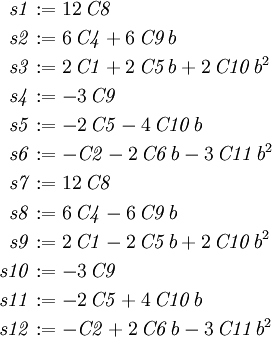

 and
and  .
.  and
and  in terms of
  ,
,  and constants. The constants can be determined from the displacement BCs applied so as to fix rigid body motion.
 , and
, and  = thickness of the beam.
 is no a linear function of
  and
and  , but St. Venant's principle can be applied.
  ) is
) is  , this prediction approaches beam theory.
 General Approach For Beam Problems
- Find the highest order polynomial terms
 and
and  for the normal and shear tractions on
  .
. - Use a polynomial of order max(
 ) excluding constant and linear terms. For example, for a polynomial of order
- Substitute (
 ) into the biharmonic equation to get a set of constraint equations. Also compute the stresses.
 - Apply boundary conditions to obtain the tractions at the boundary.
- For the strong BCs, find the coefficients of powers of x and y and equate with expressions for the tractions.
- For the weak BCs, find algebraic expressions.
- Solve the set of equations and back-substitute.