Introduction to Elasticity/Kinematics example 4
< Introduction to ElasticityExample 4
Given:
Displacement field  .
.
Find:
- The Lagrangian Green strain tensor
 .
. - The infinitesimal strain tensor
 .
. - The infintesimal rotation tensor
 .
. - The infinitesimal rotation vector
 .
. - The exact longitudinal strain in the reference material direction
 .
. - The approximate longitudinal strain in the direction based on the infinitesimal strain tensor .
Solution
The Maple output of the computations are shown below:
  with(linalg): with(LinearAlgebra):
  X := array(1..3): x := array(1..3):
  e1 := array(1..3,[1,0,0]):
  e2 := array(1..3,[0,1,0]):
  e3 := array(1..3,[0,0,1]):
  u := evalm(k*X[2]*e1 + k*X[1]*e2);
![u := \left[ \! k\,{X_{2}}, \,k\,{X_{1}}, \,0 \! \right]](../I/m/d5fe36e7d86c643706dc3e3cb71b1497.png)
x := evalm(u + X);
![x := \left[ \! k\,{X_{2}} + {X_{1}}, \,k\,{X_{1}} + {X_{2}}, \, {X_{3}} \! \right]](../I/m/f7cb96351685d9682304b04d47c2065d.png)
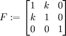
  F := linalg[matrix](3,3):
  for i from 1 to 3 do
    for j from 1 to 3 do
      F[i,j] := diff(x[i],X[j]);
    end do;
  end do;
  evalm(F);
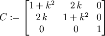
  Id := IdentityMatrix(3): C := evalm(transpose(F)&*F);
  E := evalm((1/2)*(C - Id));
![E :=
\begin{bmatrix}
{ \frac {k^{2}}{2}} & k & 0 \\ [2ex]
k & { \frac {k^{2}}{2}} & 0 \\ [2ex]
0 & 0 & 0
\end{bmatrix}](../I/m/6f05cfa01807c9d488659ee017f0a45d.png)
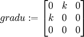
  gradu := linalg[matrix](3,3):
  for i from 1 to 3 do
    for j from 1 to 3 do
      gradu[i,j] := diff(u[i],X[j]);
    end do;
  end do;
  evalm(gradu);
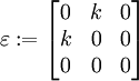
epsilon := evalm((1/2)*(gradu + transpose(gradu)));
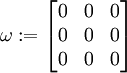
omega := evalm((1/2)*(gradu - transpose(gradu)));
  stretch1 :=  sqrt(evalm(evalm(e1&*C)&*transpose(e1))[1,1]):
  longStrain1 := stretch1 - 1;


approxLongStrain1 := evalm(evalm(e1&*epsilon)&*transpose(e1))[1,1];
The geometrical difference between the large strain and small strain cases can be observed by looking at the figures from the previous examples.
This article is issued from Wikiversity - version of the Monday, February 01, 2016. The text is available under the Creative Commons Attribution/Share Alike but additional terms may apply for the media files.