Introduction to Elasticity/Kinematics example 2

Example 2

Given: A body occupies the unit cube $X_i \in [0,1]$ in the reference configuration. The mapping between the current and the reference configuration given by $x_1 = X_1 + \kappa~X_2$ , $x_2 = X_2\,$ , $x_3 = X_3\,$ .

Find:

Sketch current configuration.
Show that motion is isochoric.
Find stretches in the directions $\widehat{\mathbf{e}}_{1}$ , $\widehat{\mathbf{e}}_{2}$ , $(1/\sqrt{2})(\widehat{\mathbf{e}}_{1}+\widehat{\mathbf{e}}_{2})$ , and $(1/\sqrt{2})(\widehat{\mathbf{e}}_{1}-\widehat{\mathbf{e}}_{2})$ .
Find the orthogonal shear strain between the reference material directions $\widehat{\mathbf{e}}_{1}$ and $\widehat{\mathbf{e}}_{2}$ . Also between directions $(1/\sqrt{2})(\widehat{\mathbf{e}}_{1}+\widehat{\mathbf{e}}_{2})$ and $(1/\sqrt{2})(\widehat{\mathbf{e}}_{1}-\widehat{\mathbf{e}}_{2})$ .
Find principal stretches and principal directions of stretch ( $\kappa = 0.4\,$ ).

Solution:

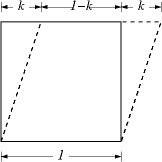Deformed shape.

All parallelograms that have the equal heights and the same base have equal areas. Hence, there is no volume change in this deformation. Hence isochoric.

Stretches in the material direction $\widehat{\mathbf{G}}$ are given by

\lambda(\widehat{\mathbf{G}}) = \sqrt{\widehat{\mathbf{G}} : \boldsymbol{C} : \widehat{\mathbf{G}}}

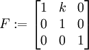
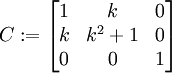
where $\boldsymbol{C}\,$ is the Cauchy-Green deformation tensor

\boldsymbol{C} = \boldsymbol{F}^T \bullet \boldsymbol{F}

We will use Maple to calculate the stretches in the four directions.


      with(linalg):
      x := array(1..3): X := array(1..3): 
      x[1] := X[1] + k*X[2]: x[2] := X[2]: x[3] := X[3]:
      F := linalg[matrix](3,3):
      for i from 1 to 3 do
        for j from 1 to 3 do
          F[i,j] := diff(x[i],X[j]); 
        end do;
      end do;
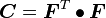
      evalm(F);
      C := evalm(transpose(F)&*F);
      e1 := linalg[matrix](1,3,[1,0,0]): 
      e2 := linalg[matrix](1,3,[0,1,0]):
      e1pe2 := evalm((e1 + e2)/sqrt(2)): 
      e1me2 := evalm((e1-e2)/sqrt(2)):''
      lambda[1] := sqrt(evalm(evalm(e1&*C)&*transpose(e1))[1,1]);
      lambda[2] := sqrt(evalm(evalm(e2&*C)&*transpose(e2))[1,1]);
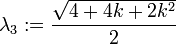
      lambda[3] := 
         simplify(sqrt(evalm(evalm(e1pe2&*C)&*transpose(e1pe2))[1,1]));
      lambda[4] :=
         simplify(sqrt(evalm(evalm(e1me2&*C)&*transpose(e1me2))[1,1]));

F := \begin{bmatrix} 1 & k & 0 \\ 0 & 1 & 0 \\ 0 & 0 & 1 \end{bmatrix}

C := \begin{bmatrix} 1 & k & 0 \\ k & k^{2} + 1 & 0 \\ 0 & 0 & 1 \end{bmatrix}

\lambda_{1} := 1 \,

\lambda_{2} := \sqrt{k^{2} + 1}

\lambda_{3} := \frac{\sqrt{4 + 4k + 2k^2}}{2}

\lambda_{4} := \frac{\sqrt{4 - 4k + 2k^2}}{2}

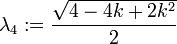
The following figure shows that the calculated stretches are correct.

Stretches

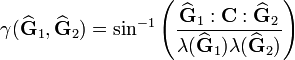
The orthogonal shear strain between two orthogonal units vectors $\widehat{\mathbf{G}}_{1}$ and $\widehat{\mathbf{G}}_{2}$ in the reference material co-ordinate system is given by

\gamma(\widehat{\mathbf{G}}_{1},\widehat{\mathbf{G}}_{2}) = \sin^{-1}\left(\frac{\widehat{\mathbf{G}}_{1}:\mathbf{C}:\widehat{\mathbf{G}}_{2}} {\lambda(\widehat{\mathbf{G}}_{1})\lambda(\widehat{\mathbf{G}}_{2})}\right)

Once again, we will use Maple to calculate these strains. The steps are the same upto the calculation of the stretches.


      numer1 := evalm(evalm(e1&*C)&*transpose(e2))[1,1]:
      denom1 := lambda[1]*lambda[2]:
      ratio1 := numer1/denom1:
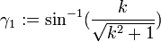
      gam1 := arcsin(ratio1);
      numer2 := simplify(evalm(evalm(e1pe2&*C)&*transpose(e1me2))[1,1]):
      denom2 := lambda[3]*lambda[4]:
      ratio2 := numer2/denom2:
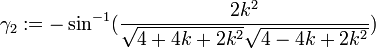
      gam2 := arcsin(ratio2);

\gamma_1 := \sin^{-1}(\frac {k}{\sqrt{k^2 + 1}})

\gamma_2 := - \sin^{-1}(\frac{2k^2}{\sqrt{4+4k+2k^2}\sqrt{4-4k+2k^2}})

The following figure shows that the calculated orthogonal shear strains are correct.

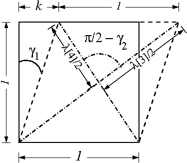Orthogonal shear strains

The value of $\gamma_{1}\,$ can easily be verified using the definition of $\sin{\gamma}\,$ . For the verification of the value of $\gamma_{2}\,$ , the cosine law

\cos(A) = \frac{b^2+c^2-a^2}{2bc}\,

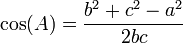
has to be used. Note that the actual length of the sides $b\,$ and $c\,$ of the triangle is obtained after multiplying the values shown in the figure by the length of the diagonal ( $\sqrt{2}$ ). Hence, the calculated values are correct.


      b := sqrt(2)/2*lambda[4]:
      c := sqrt(2)/2*lambda[3]:
      a := 1:
      A := (b^2 + c^2 - a^2)/(2*b*c);

A := \frac{2k^2}{\sqrt{4+4k+2k^2}\sqrt{4-4k+2k^2}}

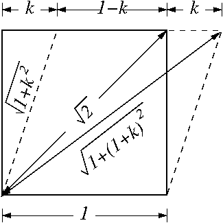
The principal stretches are given by the square roots of the eigenvalues of $\boldsymbol{C}$ . The principal directions are the eigenvectors of $\boldsymbol{C}$ .

Once again, we use Maple for our calculations.


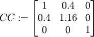
      CC := linalg[matrix](3,3):
      for i from 1 to 3 do
        for j from 1 to 3 do
          CC[i,j] := eval(C[i,j], k=0.4);
        end do;
      end do;
      evalm(CC);
      eigvals := eigenvals(CC);
      PrinStretch[1] := sqrt(eigvals[1]);
      PrinStretch[2] := sqrt(eigvals[2]);
      PrinStretch[3] := sqrt(eigvals[3]);
      PrinDir := eigenvects(CC);

CC :=\begin{bmatrix} 1 & 0.4 & 0 \\ 0.4 & 1.16 & 0 \\ 0 & 0 & 1 \end{bmatrix}

\text{eigvals} := 0.67, 1.0, 1.49

\text{PrinStretch}[1] := 0.82 ~,~~ \text{PrinStretch}[2] := 1.0 ~,~~ \text{PrinStretch}[3] := 1.22

\text{PrinDir}[1] := [0.77, -0.63, 0.] ~;~~ \text{PrinDir}[2] := [0, 0, 1] ~;~~ \text{PrinDir}[3] := [0.63, 0.77, 0.]

This article is issued from Wikiversity - version of the Monday, February 01, 2016. The text is available under the Creative Commons Attribution/Share Alike but additional terms may apply for the media files.