Introduction to Elasticity/Fourier series solutions

Using the Airy Stress Function : Fourier Series Solutions

Useful for more general boundary conditions.

Suppose

\varphi = f(x_2) \cos(\lambda x_1) ~~=or= ~~ \varphi = f(x_2) \sin(\lambda x_1)

Substitute into the biharmonic equation. Then,

f(x_2) = (A + Bx_2)e^{\lambda x_2} + (C + Dx_2)e^{-\lambda x_2}

or, equivalently,

f(x_2) = (A + Bx_2)\cosh{\lambda x_2} + (C + Dx_2)\sinh{\lambda x_2} \,

The hyperbolic form allows us to take advantage of symmetry about the $x_2 = 0$ plane.

If $\varphi = f(x_2) \cos(\lambda x_1)$ ,

\sigma_{11} = -\lambda^2 f(x_2) \cos(\lambda x_1) ~;~~ \sigma_{22} = f^{''}(x_2) \cos(\lambda x_1) ~;~~ \sigma_{12} = \lambda f^{'}(x_2) \sin(\lambda x_1)

Example of Fourier Series Technique

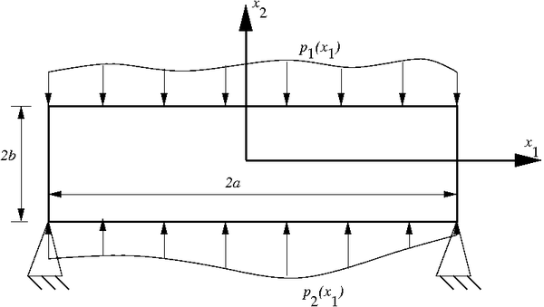Bending of an elastic beam on a foundation

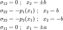
The traction boundary conditions are

\begin{align} \sigma_{12} & = 0 ~;~~ x_2 = \pm b \\ \sigma_{22} & = -p_1(x_1) ~;~~ x_2 = b \\ \sigma_{22} & = -p_2(x_1) ~;~~ x_2 = -b \\ \sigma_{11} & = 0 ~;~~ x_1 = \pm a \end{align}

The problem is broken up into four subproblems which are superposed. The subproblems are chosen so that the even/odd properties of hyperbolic functions can be exploited.

The loads for the four subproblems are chosen to be

\begin{align} f_1(x_1) = f_1(-x_1) & = \cfrac{1}{4}\left[p_1(x_1)+p_1(-x_1)+p_2(x_1)+p_2(-x_1)\right]\\ f_2(x_1) = -f_2(-x_1) & = \cfrac{1}{4}\left[p_1(x_1)-p_1(-x_1)+p_2(x_1)-p_2(-x_1)\right]\\ f_3(x_1) = f_3(-x_1) & = \cfrac{1}{4}\left[p_1(x_1)+p_1(-x_1)-p_2(x_1)-p_2(-x_1)\right]\\ f_4(x_1) = -f_4(-x_1) & = \cfrac{1}{4}\left[p_1(x_1)-p_1(-x_1)-p_2(x_1)+p_2(-x_1)\right] \end{align}

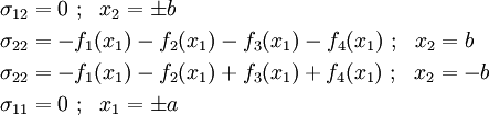
The new boundary conditions are

\begin{align} \sigma_{12} & = 0 ~;~~ x_2 = \pm b \\ \sigma_{22} & = -f_1(x_1)-f_2(x_1)-f_3(x_1)-f_4(x_1) ~;~~ x_2 = b \\ \sigma_{22} & = -f_1(x_1)-f_2(x_1)+f_3(x_1)+f_4(x_1) ~;~~ x_2 = -b \\ \sigma_{11} & = 0 ~;~~ x_1 = \pm a \end{align}

Let us look at the subproblem with loads $\pm f_3(x_1)$ applied on the top and bottom of the beam. The problem is even in $x_1$ and odd in $x_2$ . So we use,

\begin{align} \varphi & = \sum^{\infty}_{n=1} f_n(x_2) \cos(\lambda_n x_1) \\ & = \sum^{\infty}_{n=1} \left[A_n x_2\cosh(\lambda_n x_2)+ B_n\sinh(\lambda_n x_2)\right]\cos(\lambda_n x_1) \end{align}

At $x_1 = a$ ,

\sigma_{11} = -\sum^{\infty}_{n=1} \lambda_n^2 f_n(x_2) \cos(\lambda_n a)

Hence $\sigma_{11} = 0$ if $\lambda_n = (2n-1)\pi/2a$ .

We can substitute $\varphi$ and express the stresses in terms of Fourier series.

Applying the boundary conditions of $x_2 = \pm b$ we get

\begin{align} \sum^{\infty}_{n=1} \left[A_n \lambda_n \cosh(\lambda_n b)+ A_n \lambda_n^2 b \sinh(\lambda_n b)+ B_n \lambda_n^2 \cosh(\lambda_n b)\right]\sin(\lambda_n x_1) & = 0\\ \sum^{\infty}_{n=1} \left[A_n \lambda_n^2 b \cosh(\lambda_n b)+ B_n \lambda_n^2 \sinh(\lambda_n b)\right]\cos(\lambda_n x_1) & = f_3(x_1) \end{align}

The first equation is satisfied if

A_m \lambda_m \cosh(\lambda_m b)+ A_m \lambda_m^2 b \sinh(\lambda_m b)+ B_m \lambda_m^2 \cosh(\lambda_m b) = 0 \qquad (1)

Integrate the second equation from $-a$ to $a$ after multiplying by $\cos(\lambda_m x_1)$ .

All the odd functions are zero, except the case where $n=m$ .

Therefore, all that remains is

\left[A_m \lambda_m^2 b \cosh(\lambda_m b)+ B_m \lambda_m^2 \sinh(\lambda_m b)\right] a = \int_{-a}^{a} f_3(x_1) \cos(\lambda_m x_1) dx_1 \qquad (2)

We can calculate $A_m$ and $B_m$ from equations (1) and (2), substitute them into the expressions for stress to get the solution.

We do the same thing for the other subproblems.

The Fourier series approach is particularly useful if we have discontinuous or point loads.

This article is issued from Wikiversity - version of the Monday, February 01, 2016. The text is available under the Creative Commons Attribution/Share Alike but additional terms may apply for the media files.