Introduction to Elasticity/Energy methods example 4

Example 4 : Bending of a cantilevered beam

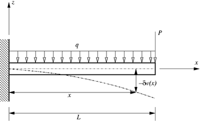Bending of a cantilevered beam

Application of the Principle of Virtual Work

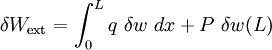
The virtual work done by the external applied forces in moving through the virtual displacement $\delta w(x)\,$ is given by

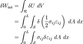
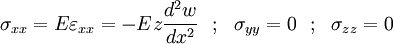
\delta W_{\text{ext}} = \int_0^L q~\delta w~dx + P~\delta w(L)

The work done by the internal forces are,

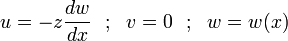
\begin{align} \delta W_{\text{int}} & = \int_{\mathcal R} \delta U~dV \\ & = \int_0^L\int_{\mathcal S}\delta\left(\frac{1}{2}\sigma_{ij}\varepsilon_{ij}\right)~dA~dx\\ & = \int_0^L\int_{\mathcal S}\sigma_{ij} \delta\varepsilon_{ij}~dA~dx \end{align}

From beam theory, the displacement field at a point in the beam is given by

u = -z\frac{dw}{dx} ~~;~~ v = 0 ~~;~~ w = w(x)

The strains are, neglecting Poisson effects,

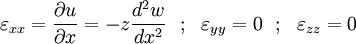
\varepsilon_{xx} = \frac{\partial u}{\partial x} = -z\frac{d^2 w}{dx^2} ~~;~~ \varepsilon_{yy} = 0 ~~;~~ \varepsilon_{zz} = 0

and the corresponding stresses are

\sigma_{xx} = E\varepsilon_{xx} = -Ez\frac{d^2 w}{dx^2} ~~;~~ \sigma_{yy} = 0 ~~;~~ \sigma_{zz} = 0

If we also neglect the shear strains and stresses, we get

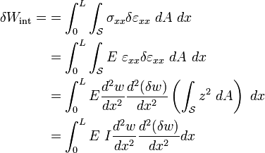
\begin{align} \delta W_{\text{int}} = & = \int_0^L\int_{\mathcal S}\sigma_{xx} \delta\varepsilon_{xx}~dA~dx \\ & = \int_0^L\int_{\mathcal S} E~\varepsilon_{xx} \delta\varepsilon_{xx}~dA~dx \\ & = \int_0^L E\frac{d^2w}{dx^2}\frac{d^2(\delta w)}{dx^2} \left(\int_{\mathcal S} z^2~dA\right)~dx \\ & = \int_0^L E~I\frac{d^2w}{dx^2}\frac{d^2(\delta w)}{dx^2} dx \end{align}

Therefore, from the principle of virtual work,

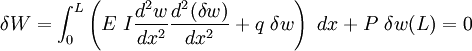
\delta W = \int_0^L \left(E~I\frac{d^2w}{dx^2}\frac{d^2(\delta w)}{dx^2} + q~\delta w\right)~dx + P~\delta w(L) = 0

Integrating by parts and after some manipulation, we get,

\begin{align} 0 &= \int_0^L \left[\frac{d^2}{dx^2}\left(E~I\frac{d^2w}{dx^2}\right) + q + P\delta(L-x)\right]\delta w~dx + \left.\left[\left(E~I\frac{d^2w}{dx^2}\right)\delta\left(\frac{dw}{dx}\right) + \frac{d}{dx}\left(E~I\frac{d^2w}{dx^2}\right)\delta w\right]\right|_0^L \end{align}

where $\delta(L-x)$ is the Dirac delta function,

\int_{-\infty}^{\infty} \delta(L-x)~f(x)~dx = f(L)

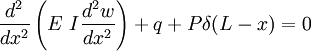
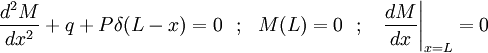
The Euler equation for the beam is, therefore,

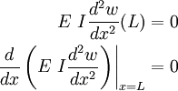
\frac{d^2}{dx^2}\left(E~I\frac{d^2w}{dx^2}\right) + q + P\delta(L-x) = 0

and the boundary conditions are

\begin{align} E~I\frac{d^2w}{dx^2}(L) & = 0 \\ \left.\frac{d}{dx}\left(E~I\frac{d^2w}{dx^2}\right)\right|_{x=L} & = 0 \end{align}

Application of the Hellinger-Prange-Reissner variational principle

The governing equations of the cantilever beam can be written as

Kinematics

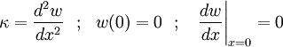
\kappa = \frac{d^2 w}{dx^2} ~~;~~ w(0) = 0 ~~;~~ \left.\frac{dw}{dx}\right|_{x=0} = 0

Constitutive Equation

M = EI\kappa

Equilibrium (kinetics)

\frac{d^2M}{dx^2} + q + P\delta(L-x) = 0 ~~;~~ M(L) = 0 ~~;~~ \left.\frac{dM}{dx}\right|_{x=L} = 0

Recall that the Hellinger-Prange-Reissner functional is given by

{\mathcal H}[s] = \int_{\mathcal{B}} U^c(\boldsymbol{\sigma}) - \int_{\mathcal{B}} \boldsymbol{\sigma}:\boldsymbol{\varepsilon}~dV - \int_{\mathcal{B}} \mathbf{f}\bullet\mathbf{u}~dV + \int_{\partial{\mathcal{B}}^{u}} \mathbf{t}\bullet(\mathbf{u}-\widehat{\mathbf{u}})~dA + \int_{\partial{\mathcal{B}}^{t}} \widehat{\mathbf{t}}\bullet\mathbf{u}~dA

If we apply the strain-displacement constraints using the Lagrange multipliers $\boldsymbol{\lambda}\,$ and the displacement boundary conditions using the Lagrange multipliers $\boldsymbol{\mu}\,$ , we get a modified functional

\bar{\mathcal H}[\mathbf{u},\boldsymbol{\varepsilon},\boldsymbol{\lambda},\boldsymbol{\mu}] = \int_{\mathcal{B}} \left[U(\boldsymbol{\varepsilon}) + \boldsymbol{\lambda}:[\frac{1}{2}(\boldsymbol{\nabla}\mathbf{u}-\boldsymbol{\nabla}\mathbf{u}^T) - \boldsymbol{\varepsilon}] - \mathbf{f}\bullet\mathbf{u}\right]~dV - \int_{\partial{\mathcal{B}}^{u}} \boldsymbol{\mu}\bullet(\mathbf{u}-\widehat{\mathbf{u}})~dA - \int_{\partial{\mathcal{B}}^{t}} \widehat{\mathbf{t}}\bullet\mathbf{u}~dA

For the cantilevered beam, the above functional becomes

\begin{align} \bar{\mathcal H}[w,\kappa,\lambda,\mu_1,\mu_2] = & \int_0^L \left[\frac{EI}{2}\kappa^2 + \left(\frac{d^2w}{dx^2}-\kappa\right)\lambda + [q + P\delta(L-x)]~w\right]~dx \\ & - M(L)\frac{dw}{dx}(L) - \frac{dM}{dx}(L)~w(L) + \mu_1[w(0) - 0] + \mu_2[\frac{dw}{dx}(0) - 0] \end{align}

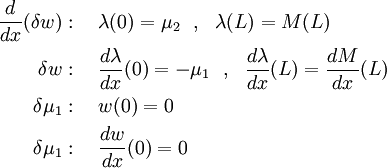
Taking the first variation of the functional, we can easily derive the Euler equations and the associated BCs.

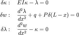
\begin{align} \delta\kappa :~~~ & EI\kappa - \lambda = 0 \\ \delta w :~~~ & \frac{d^2\lambda}{dx^2} + q + P\delta(L-x) = 0 \\ \delta\lambda :~~~ & \frac{d^2 w}{dx^2} -\kappa = 0 \end{align}

and

\begin{align} \frac{d}{dx}(\delta w) :~~~ & \lambda(0) = \mu_2 ~~,~~ \lambda(L) = M(L)\\ \delta w :~~~ & \frac{d\lambda}{dx}(0) = -\mu_1 ~~,~~ \frac{d\lambda}{dx}(L) = \frac{dM}{dx}(L)\\ \delta\mu_1 :~~~ & w(0) = 0 \\ \delta\mu_1 :~~~ & \frac{dw}{dx}(0) = 0 \end{align}

The same process can be used to derive Euler equations using the Hu-Washizu variational principle.

This article is issued from Wikiversity - version of the Monday, February 01, 2016. The text is available under the Creative Commons Attribution/Share Alike but additional terms may apply for the media files.