Introduction to Elasticity/Energy methods example 2

Example 2

Given:

The potential energy functional for a membrane stretched over a simply connected region $\mathcal{S}$ of the $x_1-x_2$ plane can be expressed as

\Pi[w(x_1,x_2)] = \frac{1}{2}\int_{\mathcal{S}} \eta\left[(w_{,1})^2 + (w_{,2})^2\right] ~dA - \int_{\mathcal S} pw~dA

where $w(x_1,x_2)$ is the deflection of the membrane, $p(x_1,x_2)$ is the prescribed transverse pressure distribution, and $\eta$ is the membrane stiffness.

Find:

The governing differential equation (Euler equation) for $w(x_1,x_2)$ on ${\mathcal S}$ .
The permissible boundary conditions at the boundary $\partial{\mathcal S}$ of ${\mathcal S}$ .

Solution

The principle of minimum potential energy requires that the functional $\Pi$ be stationary for the actual displacement field $w(x_1,x_2)$ . Taking the first variation of $\Pi$ , we get

\delta\Pi = \frac{\eta}{2}\int_{\mathcal S} \left[(2 w_{,1})\delta w_{,1} + (2 w_{,2})\delta w_{,2}\right] ~dA - \int_{\mathcal S} p~\delta w~dA

or,

\delta\Pi = \eta\int_{\mathcal S} \left[w_{,1}~\delta w_{,1} + w_{,2}~\delta w_{,2}\right] ~dA - \int_{\mathcal S} p~\delta w~dA

Now,

\begin{align} (w_{,1}~\delta w)_{,1} & = w_{,11}~\delta w + w_{,1}~\delta w_{,1} \\ (w_{,2}~\delta w)_{,2} & = w_{,22}~\delta w + w_{,2}~\delta w_{,2} \end{align}

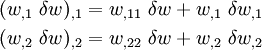
Therefore,

w_{,1}~\delta w_{,1} + w_{,2}~\delta w_{,2} = (w_{,1}~\delta w)_{,1} - w_{,11}~\delta w + (w_{,2}~\delta w)_{,2} - w_{,22}~\delta w

Plugging into the expression for $\delta\Pi$ ,

\delta\Pi = \eta\int_{\mathcal S} \left[(w_{,1}~\delta w)_{,1} + (w_{,2}~\delta w)_{,2} - (w_{,11} + w_{,22})~\delta w\right]~dA - \int_{\mathcal S} p~\delta w~dA

or,

\delta\Pi = \eta\int_{\mathcal S} \left[(w_{,1}~\delta w)_{,1} + (w_{,2}~\delta w)_{,2}\right]~dA - \eta\int_{\mathcal S} \nabla^2{w}~\delta w~dA - \int_{\mathcal S} p~\delta w~dA

Now, the Green-Riemann theorem states that

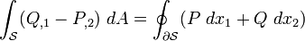
\int_{\mathcal S} (Q_{,1} - P_{,2})~dA = \oint_{\partial{\mathcal S}} (P~dx_1 + Q~dx_2)

Therefore,

\delta\Pi = \eta\oint_{\partial{\mathcal S}} \left[(w_{,1}~\delta w)~dx_2 - (w_{,2}~\delta w)~dx_1\right] - \int_{\mathcal S}\left[\eta\nabla^2{w}+p\right]~\delta w~dA

or,

\delta\Pi = \eta\oint_{\partial{\mathcal S}} \left[w_{,1}~\frac{dx_2}{ds} - w_{,2}~\frac{dx_1}{ds}\right]\delta w~ds - \int_{\mathcal S}\left[\eta\nabla^2{w}+p\right]~\delta w~dA

where $s$ is the arc length around $\partial{\mathcal S}$ .

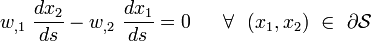
The potential energy function is rendered stationary if $\delta\Pi = 0$ . Since $\delta w$ is arbitrary, the condition of stationarity is satisfied only if the governing differential equation for $w(x_1,x_2)$ on ${\mathcal S}$ is

{ \eta\nabla^2{w}+p = 0 ~~~~~\forall~~(x_1,x_2)~\in~{\mathcal S} }

The associated boundary conditions are

{ w_{,1}~\frac{dx_2}{ds} - w_{,2}~\frac{dx_1}{ds} = 0 ~~~~~\forall~~(x_1,x_2)~\in~\partial{\mathcal S} }

This article is issued from Wikiversity - version of the Monday, February 01, 2016. The text is available under the Creative Commons Attribution/Share Alike but additional terms may apply for the media files.