Introduction to Elasticity/Constitutive relations

Constitutive relations

Any problem in elasticity is usually set up with the following components:

A strain-displacement relation.
A traction-stress relation.
Balance laws for linear and angular momentum in terms of the stress.

To close the system of equations, we need a relation between the stresses and strains. Such a relation is called a constitutive equation.

Isotropic elasticity

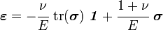
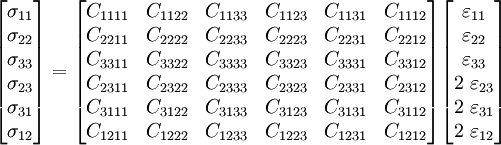
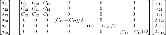
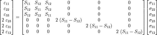
The most popular form of the constitutive relation for linear elasticity (see, for example, Strength of materials) is the following relation that holds for isotropic materials:

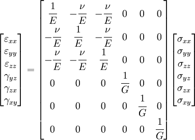
\begin{bmatrix} \varepsilon_{xx} \\ \varepsilon_{yy} \\ \varepsilon_{zz} \\ \gamma_{yz} \\ \gamma_{zx} \\ \gamma_{xy} \end{bmatrix} = \begin{bmatrix} \cfrac{1}{E} & -\cfrac{\nu}{E} & -\cfrac{\nu}{E} & 0 & 0 & 0 \\ -\cfrac{\nu}{E} & \cfrac{1}{E} & -\cfrac{\nu}{E} & 0 & 0 & 0 \\ -\cfrac{\nu}{E} & -\cfrac{\nu}{E} & \cfrac{1}{E} & 0 & 0 & 0 \\ 0 & 0 & 0 & \cfrac{1}{G} & 0 & 0 \\ 0 & 0 & 0 & 0 & \cfrac{1}{G} & 0 \\ 0 & 0 & 0 & 0 & 0 & \cfrac{1}{G} \end{bmatrix} \begin{bmatrix} \sigma_{xx} \\ \sigma_{yy} \\ \sigma_{zz} \\ \sigma_{yz} \\ \sigma_{zx} \\ \sigma_{xy} \end{bmatrix}

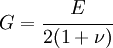
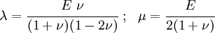
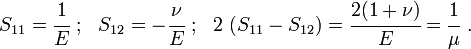
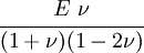
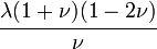
where $E$ is the Young's modulus, $\nu$ is the Poisson's ratio and $G$ is the shear modulus. The shear modulus can be expressed in terms of the Young's modulus and Poisson's ratio as

G = \cfrac{E}{2(1+\nu)}

The shear modulus is also often represented by the symbol $\mu$ . We will use $G$ and $\mu$ interchangeably in this discussion.

Engineering shear strain and tensorial shear strain

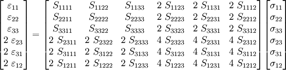
In the above matrix equation we have used $\gamma_{ij}$ to represent the shear strains rather that $\varepsilon_{ij}$ . You should keep in mind that

\gamma_{ij} = 2~\varepsilon_{ij}

An alternative form of the stress-strain relation

An alternative form of the isotropic linear elastic stress-strain relation that is easier to work with is:

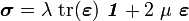
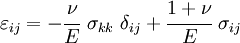
\boldsymbol{\sigma} = \lambda~\text{tr}(\boldsymbol{\varepsilon})~\boldsymbol{\mathit{1}} + 2~\mu~\boldsymbol{\varepsilon}

or, in index notation,

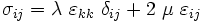
\sigma_{ij} = \lambda~\varepsilon_{kk}~\delta_{ij} + 2~\mu~\varepsilon_{ij}

Here $\lambda$ is the Lamé modulus and $\mu$ is the shear modulus. In terms of $E$ and $\nu$ :

\lambda = \cfrac{E~\nu}{(1+\nu)(1-2\nu)} ~;~~ \mu = \cfrac{E}{2(1+\nu)}

The inverse relationship is

\boldsymbol{\varepsilon} = -\cfrac{\nu}{E}~\text{tr}(\boldsymbol{\sigma})~\boldsymbol{\mathit{1}} + \cfrac{1+\nu}{E}~\boldsymbol{\sigma}

or, in index notation,

\varepsilon_{ij} = -\cfrac{\nu}{E}~\sigma_{kk}~\delta_{ij} + \cfrac{1+\nu}{E}~\sigma_{ij}

The stiffness and compliance tensors

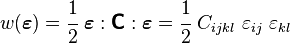
For hyperelastic materials, the stress and strain of a linear elastic material are such that one can be derived from a stored energy potential function of the other (also called a strain energy density function). Therefore, we can define an elastic material to be one which satisfies

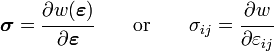
\boldsymbol{\sigma} = \cfrac{\partial w(\boldsymbol{\varepsilon})}{\partial \boldsymbol{\varepsilon}} \qquad \text{or} \qquad \sigma_{ij} = \cfrac{\partial w}{\partial \varepsilon_{ij}}

where $w$ is the strain energy density function.

If the material, in addition to being elastic, also has a linear stress-strain relation then we can write

\boldsymbol{\sigma} = \boldsymbol{\mathsf{C}}:\boldsymbol{\varepsilon} \qquad \text{or} \qquad \sigma_{ij} = C_{ijkl}~\varepsilon_{kl}

The quantity $\boldsymbol{\mathsf{C}}$ is called the stiffness tensor or the elasticity tensor.

Therefore, the strain energy density function has the form (this form is called a quadratic form)

w(\boldsymbol{\varepsilon}) = \cfrac{1}{2}~\boldsymbol{\varepsilon}:\boldsymbol{\mathsf{C}}:\boldsymbol{\varepsilon} = \cfrac{1}{2}~C_{ijkl}~\varepsilon_{ij}~ \varepsilon_{kl}

Clearly, the elasticity tensor has 81 components (think of a $9 \times 9$ matrix because the stresses and strains have nine components each). However, the symmetries of the stress tensor implies that

C_{ijkl} = C_{jikl}\,

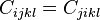
This reduces the number independent components of $C_{ijkl}\,$ to 54 (6 components for the $ij$ term and 3 each for the $k, l$ terms.

Similarly, using the symmetry of the strain tensor we can show that

C_{ijkl} = C_{ijlk}\,

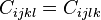
These are called the minor symmetries of the elasticity tensor and we are then left with only 36 components that are independent.

Since the strain energy function should not change when we interchange $ij$ and $kl$ in the quadratic form, we must have

C_{ijkl} = C_{klij}\,

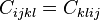
This reduces the number of independent constants to 21 (think of a symmetric $6 \times 6$ matrix). These are called the major symmetries of the stiffness tensor.

The inverse relation between the strain and the stress can be determined by taking the inverse of stress-strain relation to get

\boldsymbol{\varepsilon} = \boldsymbol{\mathsf{S}}:\boldsymbol{\sigma} \qquad \text{or} \qquad \varepsilon_{ij} = S_{ijkl}~\sigma_{kl}

where $\boldsymbol{\mathsf{S}}$ is the compliance tensor. The compliance tensor also has 21 components and the same symmetries as the stiffness tensor.

Voigt notation

To express the general stress-strain relation for a linear elastic material in terms of matrices (as we did for the isotropic elastic material) we use what is called the Voigt notation.

In this notation, the stress and strain are expressed as $6 \times 1$ column vectors and the elasticity tensor is expressed as a symmetric $6 \times 6$ matrix as shown below.

\begin{bmatrix} \sigma_{11} \\ \sigma_{22} \\ \sigma_{33} \\ \sigma_{23} \\ \sigma_{31} \\ \sigma_{12} \end{bmatrix} = \begin{bmatrix} C_{1111} & C_{1122} & C_{1133} & C_{1123} & C_{1131} & C_{1112} \\ C_{2211} & C_{2222} & C_{2233} & C_{2223} & C_{2231} & C_{2212} \\ C_{3311} & C_{3322} & C_{3333} & C_{3323} & C_{3331} & C_{3312} \\ C_{2311} & C_{2322} & C_{2333} & C_{2323} & C_{2331} & C_{2312} \\ C_{3111} & C_{3122} & C_{3133} & C_{3123} & C_{3131} & C_{3112} \\ C_{1211} & C_{1222} & C_{1233} & C_{1223} & C_{1231} & C_{1212} \end{bmatrix} \begin{bmatrix} \varepsilon_{11}\\ \varepsilon_{22}\\ \varepsilon_{33}\\ 2~\varepsilon_{23}\\ 2~\varepsilon_{31}\\ 2~\varepsilon_{12} \end{bmatrix}

\mathbf{\sigma} = \mathbf{C}~\mathbf{\varepsilon}

The inverse relation is

\begin{bmatrix} \varepsilon_{11}\\ \varepsilon_{22}\\ \varepsilon_{33}\\ 2~\varepsilon_{23}\\ 2~\varepsilon_{31}\\ 2~\varepsilon_{12} \end{bmatrix} = \begin{bmatrix} S_{1111} & S_{1122} & S_{1133} & 2~S_{1123} & 2~S_{1131} & 2~S_{1112} \\ S_{2211} & S_{2222} & S_{2233} & 2~S_{2223} & 2~S_{2231} & 2~S_{2212} \\ S_{3311} & S_{3322} & S_{3333} & 2~S_{3323} & 2~S_{3331} & 2~S_{3312} \\ 2~S_{2311} & 2~S_{2322} & 2~S_{2333} & 4~S_{2323} & 4~S_{2331} & 4~S_{2312} \\ 2~S_{3111} & 2~S_{3122} & 2~S_{3133} & 4~S_{3123} & 4~S_{3131} & 4~S_{3112} \\ 2~S_{1211} & 2~S_{1222} & 2~S_{1233} & 4~S_{1223} & 4~S_{1231} & 4~S_{1212} \end{bmatrix} \begin{bmatrix} \sigma_{11} \\ \sigma_{22} \\ \sigma_{33} \\ \sigma_{23} \\ \sigma_{31} \\ \sigma_{12} \end{bmatrix}

\mathbf{\varepsilon} = \mathbf{S}~\mathbf{\sigma}

We can show that

{\mathbf{S}} = {\mathbf{C}}^{-1}

Isotropic materials

We have already seen the matrix form of the stress-strain equation for isotropic linear elastic materials. In this case the stiffness tensor has only two independent components because every plane is a plane of elastic symmetry. In direct tensor notation

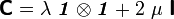
\boldsymbol{\mathsf{C}} = \lambda~\boldsymbol{\mathit{1}}\otimes\boldsymbol{\mathit{1}} + 2~\mu~\boldsymbol{\mathsf{I}}

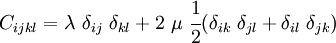
where $\lambda$ and $\mu$ are the elastic constants that we defined before, $\boldsymbol{\mathit{1}}$ is the second-order identity tensor, and $\boldsymbol{\mathsf{I}}$ is the symmetric fourth-order identity tensor. In index notation

C_{ijkl} = \lambda~\delta_{ij}~\delta_{kl} + 2~\mu~\cfrac{1}{2}(\delta_{ik}~\delta_{jl} + \delta_{il}~\delta_{jk})

You could alternatively express this equation in terms of the Young's modulus ( $E$ ) and the Poisson's ratio ( $\nu$ ) or in terms of the bulk modulus ( $K$ ) and the shear modulus ( $\mu$ ) or any other combination of two independent elastic parameters.

In Voigt notation the expression for the stress-strain law for isotropic materials can be written as

\begin{bmatrix} \sigma_{11} \\ \sigma_{22} \\ \sigma_{33} \\ \sigma_{23} \\ \sigma_{31} \\ \sigma_{12} \end{bmatrix} = \begin{bmatrix} C_{11} & C_{12} & C_{12} & 0 & 0 & 0 \\ C_{12} & C_{11} & C_{12} & 0 & 0 & 0 \\ C_{12} & C_{12} & C_{11} & 0 & 0 & 0 \\ 0 & 0 & 0 & (C_{11}-C_{12})/2 & 0 & 0 \\ 0 & 0 & 0 & 0 & (C_{11}-C_{12})/2 & 0 \\ 0 & 0 & 0 & 0 & 0 & (C_{11}-C_{12})/2 \end{bmatrix} \begin{bmatrix} \varepsilon_{11}\\ \varepsilon_{22}\\ \varepsilon_{33}\\ 2~\varepsilon_{23}\\ 2~\varepsilon_{31}\\ 2~\varepsilon_{12} \end{bmatrix}

where

C_{11} = \cfrac{E~(1-\nu)}{(1+\nu)(1-2\nu)} ~;~~ C_{12} = \cfrac{E~\nu}{(1+\nu)(1-2\nu)} ~;~~ (C_{11}-C_{12})/2 = \cfrac{E}{2(1+\nu)} = \mu ~.

The Voigt form of the strain-stress relation can be written as

\begin{bmatrix} \varepsilon_{11}\\ \varepsilon_{22}\\ \varepsilon_{33}\\ 2~\varepsilon_{23}\\ 2~\varepsilon_{31}\\ 2~\varepsilon_{12} \end{bmatrix} = \begin{bmatrix} S_{11} & S_{12} & S_{12} & 0 & 0 & 0 \\ S_{12} & S_{11} & S_{12} & 0 & 0 & 0 \\ S_{12} & S_{12} & S_{11} & 0 & 0 & 0 \\ 0 & 0 & 0 & 2~(S_{11}-S_{12}) & 0 & 0 \\ 0 & 0 & 0 & 0 & 2~(S_{11}-S_{12}) & 0 \\ 0 & 0 & 0 & 0 & 0 & 2~(S_{11}-S_{12}) \end{bmatrix} \begin{bmatrix} \sigma_{11} \\ \sigma_{22} \\ \sigma_{33} \\ \sigma_{23} \\ \sigma_{31} \\ \sigma_{12} \end{bmatrix}

where

S_{11} = \cfrac{1}{E} ~;~~ S_{12} = -\cfrac{\nu}{E} ~;~~ 2~(S_{11}-S_{12}) = \cfrac{2(1+\nu)}{E} = \cfrac{1}{\mu} ~.

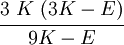
The relations between various moduli are shown in the table below:

	$\mu, \nu$	$\nu, \lambda$	$\mu, \lambda$	$K, \lambda$	$\mu, E$	$\mu, K$	$\nu, E$	$\nu, K$	$K, E$
$\lambda$	$\cfrac{2~\mu~\nu}{1-2\nu}$	-	-	-	$\cfrac{\mu~(E - 2\mu)}{3\mu - E}$	$K - \cfrac{2}{3}~\mu$	$\cfrac{E~\nu}{(1+\nu)(1-2\nu)}$	$\cfrac{3~K~\nu}{1+\nu}$	$\cfrac{3~K~(3K- E)}{9K - E}$
$\mu$	-	$\cfrac{\lambda~(1-2\nu)}{2\nu}$	-	$\cfrac{3}{2} (K - \lambda)$	-	-	$\cfrac{E}{2(1+\nu)}$	$\cfrac{3K(1-2\nu)}{2(1+\nu)}$	$\cfrac{3KE}{9K - E}$
$\nu$	-	-	$\cfrac{\lambda}{2(\lambda+\mu)}$	$\cfrac{\lambda}{3K- \lambda}$	$\cfrac{E-2\mu}{2\mu}$	$\cfrac{3K-2\mu}{2(3K+\mu)}$	-	-	$\cfrac{3K-E}{6K}$
$E$	$2\mu(1+\nu)$	$\cfrac{\lambda(1+\nu)(1-2\nu)}{\nu}$	$\cfrac{\mu(3\lambda+2\mu)}{\lambda+\mu}$	$\cfrac{9K(K-\lambda)}{3K-\lambda}$	-	$\cfrac{9K\mu}{3K + \mu}$	-	$3K(1-2\nu)$	-
$K$	$\cfrac{2\mu(1+\nu)}{3(1-2\nu)}$	$\cfrac{\lambda(1+\nu)}{3\nu}$	$\lambda + \cfrac{2}{3}~\mu$	-	$\cfrac{\mu E}{3(3\mu - E)}$	-	$\cfrac{E}{3(1-2\nu)}$	-	-

This article is issued from Wikiversity - version of the Wednesday, October 07, 2015. The text is available under the Creative Commons Attribution/Share Alike but additional terms may apply for the media files.