Introduction to Elasticity/Antiplane shear example 1

Example 1

Given:

The body $-\alpha < \theta < \alpha$ , $0 \le r < a$ is supported at $r = a$ and loaded only by a uniform antiplane shear traction $\sigma_{\theta z} = S$ on the surface $\theta = \alpha$ , the other surface being traction-free.

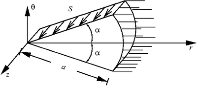A body loaded in antiplane shear

Find:

Find the complete stress field in the body, using strong boundary conditions on $\theta = \pm\alpha$ and weak conditions on $r = a$ .

[Hint: Since the traction $\sigma_{\theta z}$ is uniform on the surface $\theta = \alpha$ , from the expression for antiplane stress we can see that the displacement varies with $r^1 = r$ . The most general solution for the equilibrium equation for this behavior is $u(r,\theta) = Ar\cos\theta + Br\sin\theta$ ]

Solution

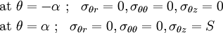
Step 1: Identify boundary conditions

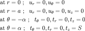
\begin{align} \text{at}~ r & = 0 ~;~~ u_r = 0, u_{\theta} = 0 \\ \text{at}~ r & = a ~;~~ u_r = 0, u_{\theta} = 0, u_{z} = 0 \\ \text{at}~ \theta & = -\alpha ~;~~ t_{\theta} = 0, t_{r} = 0, t_{z} = 0 \\ \text{at}~ \theta & = \alpha ~;~~ t_{\theta} = 0, t_{r} = 0, t_{z} = S \end{align}

The traction boundary conditions in terms of components of the stress tensor are

\begin{align} \text{at}~ \theta & = -\alpha ~;~~ \sigma_{\theta r} = 0, \sigma_{\theta\theta} = 0, \sigma_{\theta z} = 0 \\ \text{at}~ \theta & = \alpha ~;~~ \sigma_{\theta r} = 0, \sigma_{\theta\theta} = 0, \sigma_{\theta z} = S \end{align}

Step 2: Assume solution

Assume that the problem satisfies the conditions required for antiplane shear. If $\sigma_{\theta z}$ is to be uniform along $\theta=\alpha$ , then

\sigma_{\theta z} = \frac{\mu}{r} \frac{\partial u_z}{\partial \theta} = C

or,

\frac{\partial u_z}{\partial \theta} = \frac{Cr}{\mu}

The general form of $u_z$ that satisfies the above requirement is

u_z(r,\theta) = Ar\cos\theta + Br\sin\theta + C

where $A$ , $B$ , $C$ are constants.

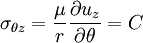
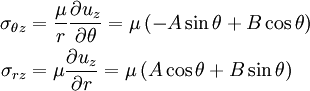
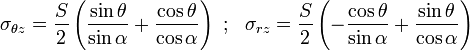
Step 3: Compute stresses

The stresses are

\begin{align} \sigma_{\theta z} & = \frac{\mu}{r} \frac{\partial u_z}{\partial \theta} = \mu \left(-A\sin\theta + B\cos\theta\right) \\ \sigma_{rz} & = \mu \frac{\partial u_z}{\partial r} = \mu \left(A\cos\theta + B\sin\theta\right) \end{align}

Step 4: Check if traction BCs are satisfied

The antiplane strain assumption leads to the $\sigma_{\theta\theta}$ and $\sigma_{r\theta}$ BCs being satisfied. From the boundary conditions on $\sigma_{\theta z}$ , we have

\begin{align} 0 & = \mu \left(A\sin\alpha + B\cos\alpha\right) \\ S & = \mu \left(-A\sin\alpha + B\cos\alpha\right) \end{align}

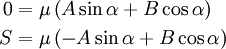
Solving,

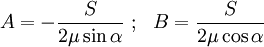
A = -\frac{S}{2\mu\sin\alpha} ~;~~ B = \frac{S}{2\mu\cos\alpha}

This gives us the stress field

\sigma_{\theta z} = \frac{S}{2} \left(\frac{\sin\theta}{\sin\alpha} + \frac{\cos\theta}{\cos\alpha}\right) ~;~~ \sigma_{rz} = \frac{S}{2} \left(-\frac{\cos\theta}{\sin\alpha} + \frac{\sin\theta}{\cos\alpha}\right)

Step 5: Compute displacements

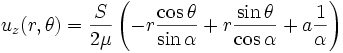
The displacement field is

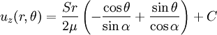
u_z(r,\theta) = \frac{Sr}{2\mu}\left(-\frac{\cos\theta}{\sin\alpha} + \frac{\sin\theta}{\cos\alpha}\right) + C

where the constant $C$ corresponds to a superposed rigid body displacement.

Step 6: Check if displacement BCs are satisfied

The displacement BCs on $u_r$ and $u_{\theta}$ are automatically satisfied by the antiplane strain assumption. We will try to satisfy the boundary conditions on $u_z$ in a weak sense, i.e, at $r = a$ ,

\int_{-\alpha}^{\alpha} u_z(a, \theta) d\theta = 0~.

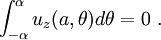
This weak condition does not affect the stress field. Plugging in $u_z$ ,

\begin{align} 0 & = \int_{-\alpha}^{\alpha} u_z(a, \theta) d\theta \\ & = \frac{Sa}{2\mu}\int_{-\alpha}^{\alpha} \left(-\frac{\cos\theta}{\sin\alpha} + \frac{\sin\theta}{\cos\alpha} + C\frac{2\mu}{Sa}\right) d\theta \\ & = \frac{Sa}{2\mu}\int_{-\alpha}^{\alpha} \left(-\frac{\cos\theta}{\sin\alpha} + \frac{\sin\theta}{\cos\alpha} + C\frac{2\mu}{Sa}\right) d\theta \\ & = \frac{Sa}{2\mu}\left[ \left(-\frac{\sin\theta}{\sin\alpha} - \frac{\cos\theta}{\cos\alpha} + C\theta\frac{2\mu}{Sa}\right) \right]_{-\alpha}^{\alpha} \\ & = \frac{Sa}{2\mu} \left(-2\frac{\sin\alpha}{\sin\alpha} + 2C\alpha\frac{2\mu}{Sa}\right) \\ & = -\frac{Sa}{\mu} + C\alpha \end{align}

Therefore,

C = \frac{Sa}{2\mu\alpha}

The approximate displacement field is

u_z(r,\theta) = \frac{S}{2\mu}\left(-r\frac{\cos\theta}{\sin\alpha} + r\frac{\sin\theta}{\cos\alpha} + a\frac{1}{\alpha}\right)

This article is issued from Wikiversity - version of the Saturday, February 13, 2016. The text is available under the Creative Commons Attribution/Share Alike but additional terms may apply for the media files.