Interpolation and Extrapolation

This course belongs to the track Numerical Algorithms in the Department of Scientific Computing in the School of Computer Science.

In this course, students will learn how to approximate discrete data. Different representations and techniques for the approximation are discussed.

Discrete Data

Discrete data arises from measurements of $f(x)$ or when $f(x)$ is difficult or expensive to evaluate.

In general, discrete data is given by a set of nodes $x_i$ , $i=1 \dots n$ and the function $f(x)$ evaluated at these points: $f_i = f(x_i)$ , $i=1 \dots n$ .

In the following, we will refer to the individual nodes and function values as $x_i$ and $f_i$ respectively. The vectors of the $n$ nodes or function values are written as $\underline{\mathbf x}$ and $\underline{\mathbf f}$ respectively.

We will also always assume that the $x_i$ are distinct.

Polynomial Interpolation

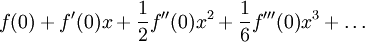
Although there are many ways of representing a function $f(x)$ , polynomials are the tool of choice for interpolation. As the Taylor series expansion of a function $f(x)$ around $0$ shows, every continuous, differentiable function has a polynomial representation

$f(x)$	$=$	$f(0) + f'(0)x + \frac{1}{2}f''(0)x^2 + \frac{1}{6}f'''(0)x^3 + \dots$
	$=$	$\sum_{n=0}^\infty \underbrace{\frac{1}{n!}f^{(n)}(0)}_{=a_n}x^n$
	$=$	$\sum_{n=0}^\infty a_n x^n$

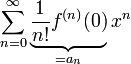
in which the $a_n = \frac{1}{n!}f^{(n)}(0)$ are the exact weights.

If a function $f(x)$ is assumed to be continuous and differentiable and we assume that it's derivatives $f^{(n)}(0)$ are zero or of negligible magnitude for increasing $n$ , it is a good idea to approximate the function with a polynomial.

Given $n$ distinct nodes $x_i$ , $i=1 \dots n$ at which the function values $f_i = f(x_i)$ are known, we can construct an interpolating polynomial $g(x)$ such that $g(x_i) = f_i$ for all $i=1 \dots n$ . Such an interpolating polynomial with degree $\le n$ is unique. However infinitely many such polynomials can be found with degree $>n\;$ .

Any nice way of deriving the interpolation error?

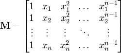
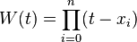
The Vandermonde Matrix

By definition as given above, our polynomial

g(x) = \sum_{i=0}^{n-1} a_i x^i

must interpolate the function $f(x)$ at the $n$ nodes $x_i$ . This leads to the following system of $n$ linear equations in the coefficients $a_i$ :

$f(x_1)$	$=$	$a_0 + a_1x_1 + a_2 x_1^2 + \dots + a_{n-1} x_1^{n-1}$
$f(x_2)$	$=$	$a_0 + a_1x_2 + a_2 x_2^2 + \dots + a_{n-1} x_2^{n-1}$
	$\vdots$
$f(x_n)$	$=$	$a_0 + a_1x_n + a_2 x_n^2 + \dots + a_{n-1} x_n^{n-1}$

We can re-write this system of linear equation in matrix notation as

\mathbf M \mathbf a = \mathbf f

where $\mathbf a$ is the vector of the $a_i$ , $i=0\dots n-1$ coefficients and $\mathbf M$ is the so-called moment matrix or Vandermonde matrix with

\mathbf M = \begin{bmatrix} 1 & x_1 & x_1^2 & \dots & x_1^{n-1} \\ 1 & x_2 & x_2^2 & \dots & x_2^{n-1} \\ \vdots & \vdots & \vdots & \ddots & \vdots \\ 1 & x_n & x_n^2 & \dots & x_n^{n-1} \end{bmatrix}

\mathbf M_{i,j} = x_i^{j-1}

This linear system of equations can be solved for $\mathbf a$ using Gauss elimination or other methods.

The following shows how this can be done in Matlab or GNU Octave.

% declare our function f
f = inline('sin(pi*2*x)','x')

% order of the interpolation?
n = 5

% declare the nodes x_i as random in [0,1]
x = rand(n,1)

% create the moment matrix
M = zeros(n)
for i=1:n
    M(:,i) = x.^(i-1);
end

% solve for the coefficients a
a = M \ f(x)

% compute g(x)
g = ones(n,1) * a(1)
for i=2:n
    g = g + x.^(i-1)*a(i);
end;

% how good was the approximation?
g - f(x)

However practical it may seem, the Vandermonde matrix is not especially suited for more than just a few nodes. Due to it's special structure, the Condition Number of the Vandermode matrix increases with $n$ .

If in the above example we set $n=10$ and compute $\mathbf a$ with

% solve for the coefficients a
a = inv(M) * f(x)

the approximation is only good up to 10 digits. For $n=20$ it is accurate only to one digit.

We must therefore consider other means of computing and/or representing $g(x)$ .

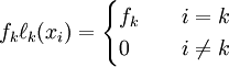
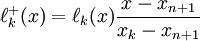
Lagrange Interpolation

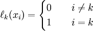
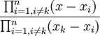
Given a set of $n$ nodes $x_i$ , $i=1 \dots n$ , we define the $k$ ^th Lagrange Polynomial as the polynomial of degree $n-1$ that satisifies

\ell_k(x_i) = \begin{cases}0\quad & i \neq k \\ 1 & i = k\end{cases}

Maybe add a nice plot of a Lagrange polynomial over a few nodes?

The first condition, namely that $\ell_k(x_i)=0$ for $i \neq k$ can be satisfied by construction. Since every polynomial of degree $n-1$ can be represented as the product

g(x) = c\prod_{i=1}^{n-1}(x - \xi_i)

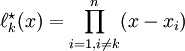
where the $\xi_i$ are the roots of $g(x)$ and $c$ is some constant, we can construct $\ell_k^\star(x)$ as

\ell_k^\star(x) = \prod_{i=1,i \neq k}^{n}(x - x_i)

The polynomial $\ell_k^\star(x)$ is of order $n-1$ and satisifies the first condition, namely that $\ell_k^\star(x_i)=0$ for $i \neq k$ .

Since, by construction, the $n-1$ roots of $\ell_k^\star(x)$ are at the nodes $x_i$ , $i \neq k$ , we know that the value of $\ell_k^\star(x_k)$ cannot be zero. This value, however, should be $1$ by definition. We can enforce this by scaling $\ell_k^\star(x)$ by $\ell_k^\star(x_k)^{-1}$ :

$\ell_k(x)$	$=$	$\frac{\ell_k^\star(x)}{\ell_k^\star(x_k)}$
	$=$	$\frac{\prod_{i=1,i \neq k}^{n}(x - x_i)}{\prod_{i=1,i \neq k}^{n}(x_k - x_i)}$

If we insert any $x_i$ , $i \neq k$ into the above equation, the nominator becomes $0$ and the first condition is satisified. If we insert $x_k$ , the nominator and the denominator are the same and we get $1$ , which means that the second condition is also satisfied.

We can now use the Lagrange polynomials $\ell_k(x)$ to construct a polynomial $g(x)$ of degree $n-1$ which interpolates the $n$ function values $f_i$ at the points $x_i$ .

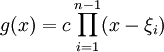
Consider that, given the definition of $\ell_k(x)$ ,

f_k\ell_k(x_i) = \begin{cases}f_k\quad & i = k \\ 0 & i \neq k\end{cases}

Therefore, if we define $g(x)$ as

g(x) = \sum_{k=1}^{n} f_k\ell_k(x)

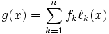
then $g(x_i) = f_i$ for all $i=1 \dots n$ . Since the $\ell_k(x)$ are all of degree $n-1$ , the weighted sum of these polynomials is also of degree $n-1$ .

Therefore, $g(x)$ is the polynomial of degree $n-1$ which interpolates the $n$ values $f_i$ at the nodes $x_i$ .

The representation with Lagrange polynomials has some advantages over the monomial representation 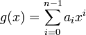$g(x)=\sum_{i=0}^{n-1}a_ix^i$ described in the previous section.

First of all, once the Lagrange polynomials have been computed over a set of nodes $x_i$ , computing the interpolating polynomial for a new set of function values $f_i$ is trivial, since these only need to be multiplied with the Lagrange polynomials, which are independent of the $f_i$ .

Another advantage is that the representation can easily be extended if additional points are added. The Lagrange polynomial $\ell_k^+(x)$ , obtained by adding a point $x_{n+1}$ to the interpolation, is

\ell_k^+(x) = \ell_k(x) \frac{x - x_{n+1}}{x_k - x_{n+1}}

Only the new polynomial $\ell_{n+1}^+(x)$ would need to be re-computed from scratch.

In the monomial representation, adding a point would involve adding an extra line and column to the Vandermonde matrix and re-computing the solution.

Add a word on Barycentric interpolation to facilitate adding points.

Newton Interpolation

Given a set of $n$ function values $f_i$ evaluated at the nodes $x_i$ , the Newton polynomial is defined as the sum

g(x) = \sum_{i=1}^{n} a_in_i(x)

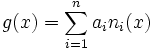
where the $n_i(x)$ are the $n$ Newton basis polynomials defined by

$n_1(x)$	$=$	$1$
$n_i(x)$	$=$	$\prod_{k=1}^{i-1} (x - x_k)\quad \mbox{for } i > 1$ .

An interpolation polynomial of degree n+1 can be easily obtained from that of degree n by just adding one more node point $x_{n+1}$ and adding a polynomial of degree n+1 to $g(x)$ .

The Newton form of the interpolating polynomial is particularly suited to computations by hand, and underlies Neville's algorithm for polynomial interpolation. It is also directly related to the exact formula for the error term $f_i - g(x_i)$ . Any good text in numerical analysis will prove this formula and fully specify Neville's algorithm, usually doing both via divided differences.

(Should link to error formula, divided differences and Neville's algorithm, adding articles where they don't exist)

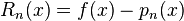
Interpolation error

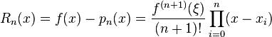
When interpolating a given function f by a polynomial of degree n at the nodes x₀,...,x_n we get the error

f(x) - p_n(x) = f[x_0,\ldots,x_n,x] \prod_{i=0}^n (x-x_i)

where

f[x_0,\ldots,x_n,x]

is the notation for divided differences.

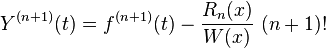
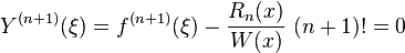
If f is n + 1 times continuously differentiable on a closed interval I and $p_n(x)$ be a polynomial of degree at most n that interpolates f at n + 1 distinct points {x_i} (i=0,1,...,n) in that interval. Then for each x in the interval there exists $\xi$ in that interval such that

f(x) - p_n(x) = \frac{f^{(n+1)}(\xi)}{(n+1)!} \prod_{i=0}^n (x-x_i)

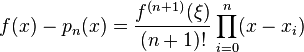
The above error bound suggests choosing the interpolation points x_i such that the product | Π (x − x_i) | is as small as possible.

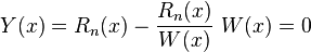
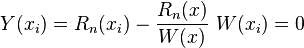
Proof

Let's set the error term is

$R_n(x) = f(x) - p_n(x)$

and set up a auxiliary function $Y(t)$ and the function is

$Y(t) = R_n(t) - \frac{R_n(x)}{W(x)} \ W(t)$

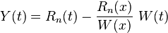
where

$W(t) = \prod_{i=0}^n (t-x_i)$

and

$W(x) = \prod_{i=0}^n (x-x_i)$

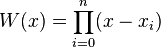
Since $x_i$ are roots of function f and $p_n(x)$ , so we will have

$Y(x) = R_n(x) - \frac{R_n(x)}{W(x)} \ W(x) = 0$

and

$Y(x_i) = R_n(x_i) - \frac{R_n(x)}{W(x)} \ W(x_i) = 0$

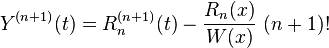
Then $Y(t)$ has n+2 roots. From Rolle's theorem, $Y^\prime(t)$ has n+1 roots, then $Y^{(n+1)}(t)$ has one root $\xi$ , where $\xi$ is in the interval I.

So we can get

$Y^{(n+1)}(t) = R_n^{(n+1)}(t) - \frac{R_n(x)}{W(x)} \ (n+1)!$

Since $p_n(x)$ is a polynomial of degree at most n, then

$R_n^{(n+1)}(t) = f^{(n+1)}(t)$

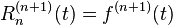
Thus

$Y^{(n+1)}(t) = f^{(n+1)}(t) - \frac{R_n(x)}{W(x)} \ (n+1)!$

Since $\xi$ is the root of $Y^{(n+1)}(t)$ , so

$Y^{(n+1)}(\xi) = f^{(n+1)}(\xi) - \frac{R_n(x)}{W(x)} \ (n+1)! = 0$

Therefore

$R_n(x) = f(x) - p_n(x) = \frac{f^{(n+1)}(\xi)}{(n+1)!} \prod_{i=0}^n (x-x_i)$ .

Piecewise Interpolation / Splines

B Splines

Extrapolation

Interpolation is the technique of estimating the value of a function for any intermediate value of the independent variable while the process of computing the value of the function outside the given range is called extrapolation.

Caution must be used when extrapolating, as assumptions outside the data region (linearization, general shape and slope) may breakdown.

This article is issued from Wikiversity - version of the Friday, October 26, 2012. The text is available under the Creative Commons Attribution/Share Alike but additional terms may apply for the media files.