Heat equation/Solution to the 2-D Heat Equation

Definition

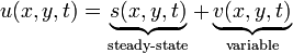
The solution to the 2-dimensional heat equation (in rectangular coordinates) deals with two spatial and a time dimension, $u(x,y,t)$ . The heat equation, the variable limits, the Robin boundary conditions, and the initial condition are defined as:

$\begin{align} u_t=k \left [ u_{xx} + u_{yy} \right ] + h(x,y,t) \\ (x,y,t) \in [0,L] \times [0,M] \times [0,\infty) \\ \alpha_1u(0,y,t)-\beta_1u_x(0,y,t)=b_1(y,t) \\ \alpha_2u(L,y,t)+\beta_2u_x(L,y,t)=b_1(y,t) \\ \alpha_3u(x,0,t)-\beta_3u_y(x,0,t)=b_1(x,t) \\ \alpha_4u(x,M,t)+\beta_4u_y(x,M,t)=b_1(x,t) \\ u(x,y,0)=f(x,y) \end{align}$

Solution

The solution is just an advanced version of the solution in 1 dimension. If you have questions about the steps shown here, review the 1-D solution.

Step 1: Partition Solution

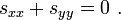
Just as in the 1-D solution, we partition the solution into a "steady-state" and a "variable" portion:

$u(x,y,t)=\underbrace{s(x,y,t)}_{ \text{steady-state} }+\underbrace{v(x,y,t)}_{ \text{variable} }$

We substitute this equation into the initial boundary value problem (IBVP):

$\begin{cases} s_t+v_t=k \left [ s_{xx}+v_{xx}+s_{yy}+v_{yy} \right ] + h(x,y,t) \\ \alpha_1s(0,y,t)+\alpha_1v(0,y,t)-\beta_1s_x(0,y,t)-\beta_1v_x(0,y,t)=b_1(y,t) \\ \alpha_2s(0,y,t)+\alpha_2v(L,y,t)+\beta_2s_x(L,y,t)+\beta_2v_x(L,y,t)=b_2(y,t) \\ \alpha_3s(x,0,t)+\alpha_3v(x,0,t)-\beta_3s_y(x,0,t)-\beta_3v_y(x,0,t)=b_3(x,t) \\ \alpha_4s(x,M,t)+\alpha_4v(x,M,t)+\beta_4s_y(x,M,t)+\beta_4v_y(x,M,t)=b_4(x,t) \\ s(x,y,0)+v(x,y,0)=f(x,y) \end{cases}$

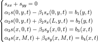
We want to set some conditions on s and v:

Let s satisfy the Laplace equation: $s_{xx}+s_{yy}=0~.$
Let s satisfy the non-homogeneous boundary conditions.
Let v satisfy the non-homogeneous equation and homogeneous boundary conditions.

We end up with 2 separate IBVPs:

$\begin{cases} s_{xx}+s_{yy}=0 \\ \alpha_1s(0,y,t)-\beta_1s_x(0,y,t)=b_1(y,t) \\ \alpha_2s(0,y,t)+\beta_2s_x(L,y,t)=b_2(y,t) \\ \alpha_3s(x,0,t)-\beta_3s_y(x,0,t)=b_3(x,t) \\ \alpha_4s(x,M,t)+\beta_4s_y(x,M,t)=b_4(x,t) \\ \end{cases}$

$\begin{cases} v_t=k \left [ v_{xx}+v_{yy} \right ] + h(x,y,t) - s_t(x,y,t) \\ \alpha_1v(0,y,t)-\beta_1v_x(0,y,t)=0 \\ \alpha_2v(L,y,t)+\beta_2v_x(L,y,t)=0 \\ \alpha_3v(x,0,t)-\beta_3v_y(x,0,t)=0 \\ \alpha_4v(x,M,t)+\beta_4v_y(x,M,t)=0 \\ v(x,y,0)=f(x,y)-s(x,y,0) \end{cases}$

Step 2: Solve Steady-State Portion

Solving for the steady-state portion is exactly like solving the Laplace equation with 4 non-homogeneous boundary conditions. Using that technique, a solution can be found for all types of boundary conditions.

Step 3: Solve Variable Portion

Step 3.1: Solve Associated Homogeneous BVP

The associated homogeneous BVP equation is:

$v_t=k \left [ v_{xx}+v_{yy} \right ]$

The boundary conditions for v are the ones in the IBVP above.

Separate Variables

$v(x,y,t)=X(x)Y(y)T(t)$

$\Rightarrow XYT'=k \lbrack X''YT+XY''T \rbrack$

$\Rightarrow \frac{T'}{kT} = \frac{X''}{X} + \frac{Y''}{Y} = \mu$

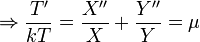
By similar methods, you obtain the following ODEs:

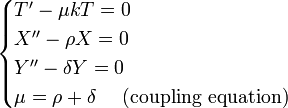
$\begin{cases} T'-\mu kT=0 \\ X''-\rho X=0 \\ Y''-\delta Y=0 \\ \mu=\rho + \delta \quad \text{ (coupling equation) } \end{cases}$

Translate Boundary Conditions

$\left . \begin{align} \left [ \alpha_1X(0)-\beta_1X'(0) \right ] Y(y)T(t) & = 0 \\ \left [ \alpha_2X(L)+\beta_2X'(L) \right ] Y(y)T(t) & = 0 \\ \left [ \alpha_3Y(0)-\beta_3Y'(0) \right ] X(x)T(t) & = 0 \\ \left [ \alpha_4Y(M)+\beta_4Y'(M) \right ] X(x)T(t) & = 0 \end{align} \right \} \Rightarrow \begin{align} \alpha_1X(0)-\beta_1X'(0) = 0 \\ \alpha_2X(L)+\beta_2X'(L) = 0 \\ \alpha_3Y(0)-\beta_3Y'(0) = 0 \\ \alpha_4Y(M)+\beta_4Y'(M) = 0 \end{align}$

Solve SLPs

$\left . \begin{align} X''-\rho X=0\\ \alpha_1X(0)-\beta_1X'(0) = 0 \\ \alpha_2X(L)+\beta_2X'(L) = 0 \end{align} \right \} \begin{align} & -\rho =\lambda^2 \\ & \text{Eigenvalues } \lambda_n \text{: solutions to equation } (\alpha_1\alpha_2-\beta_1\beta_2\lambda^2) \sin (\lambda L) + (\alpha_1\beta_2+\alpha_2\beta_1)\lambda \cos (\lambda L)=0 \\ & X_n(x)=\beta_1\lambda_n \cos (\lambda_n x) + \alpha_1 \sin (\lambda_n x), n=0,1,2,\cdots \end{align}$

$\left . \begin{align} Y''-\delta Y=0 \\ \alpha_3Y(0)-\beta_3Y'(0) = 0 \\ \alpha_4Y(M)+\beta_4Y'(M) = 0 \end{align} \right \} \begin{align} & -\delta =\hat \lambda^2 \ \\ & \text{Eigenvalues } \hat{\lambda}_m \text{: solutions to equation } (\alpha_3\alpha_4-\beta_3\beta_4 \hat{\lambda}^2) \sin (\hat{\lambda}M ) + (\alpha_3\beta_4+\alpha_4\beta_3) \hat{\lambda} \cos ( \hat{\lambda} M)=0 \\ & Y_m(x)=\beta_3 (\hat{\lambda}_m ) \cos ( \hat{\lambda}_m y) + \alpha_3 \sin ( \hat{\lambda}_m y), m=0,1,2,\cdots \end{align}$

We have obtained eigenfunctions that we can use to solve the nonhomogeneous IBVP.

Step 3.2: Solve Non-homogeneous IBVP

Setup Problem

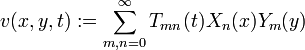
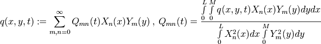
Just like in the 1-D case, we define v(x,y,t) and q(x,y,t) as infinite sums:

$v(x,y,t):=\sum_{m,n=0}^\infty T_{mn}(t)X_n(x)Y_m(y)$

$q(x,y,t):=\sum_{m,n=0}^\infty Q_{mn}(t)X_n(x)Y_m(y)~,~Q_{mn}(t)=\frac{\int\limits_0^L \int\limits_0^M q(x,y,t)X_n(x)Y_m(y) dy dx}{\int\limits_0^L X_n^2(x) dx \int\limits_0^M Y_m^2(y) dy}$

Determine Coefficients

We then substitute expansion into the PDE:

$\frac{\partial}{\partial t} \left [ \sum T_{mn}(t)X_n(x)Y_m(y) \right ] = k \left \{ \frac{\partial}{\partial x^2} \left [ \sum T_{mn}(t)X_n(x)Y_m(y) \right ] + \frac{\partial}{\partial y^2} \left [ \sum T_{mn}(t)X_n(x)Y_m(y) \right ] \right \} + \sum Q_{mn}(t)X_n(x)Y_m(y)$

$\Rightarrow \sum T_{mn}'(t)X_n(x)Y_m(y) = k \left \{ \sum T_{mn}(t)X_n''(x)Y_m(y) + \sum T_{mn}(t)X_n(x)Y_m''(y) \right \} + \sum Q_{mn}(t)X_n(x)Y_m(y)$

$\Rightarrow \sum T_{mn}'(t)X_n(x)Y_m(y) = \sum k \left \{ T_{mn}(t)[-\lambda_n^2X_n(x)]Y_m(y) + \sum T_{mn}(t)X_n(x)[-\hat{\lambda}_m^2Y_m(y)] \right \} + \sum Q_{mn}(t)X_n(x)Y_m(y)$

$\Rightarrow \sum \left [ T_{mn}'(t)+k(\lambda_n^2+\hat{\lambda}_m^2) \right ] X_n(x)Y_m(y) = \sum Q_{mn}(t)X_n(x)Y_m(y)$

This implies that $X_n(x) \otimes Y_m(y)~$ forms an orthogonal basis. This means that we can write the following:

$\Rightarrow T_{mn}'(t)+k(\lambda_n^2+\hat{\lambda}_m^2)=Q_{mn}(t)$

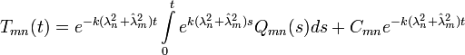
This is a first-order ODE which can be solved using the integration factor:

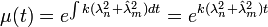
$\mu(t)=e^{\int k(\lambda_n^2+\hat{\lambda}_m^2) dt}=e^{k(\lambda_n^2+\hat{\lambda}_m^2)t}$

Solving for our coefficient we get:

$T_{mn}(t)=e^{-k(\lambda_n^2+\hat{\lambda}_m^2)t} \int\limits_0^t e^{k(\lambda_n^2+\hat{\lambda}_m^2)s} Q_{mn}(s) ds + C_{mn}e^{-k(\lambda_n^2+\hat{\lambda}_m^2)t}$

Satisfy Initial Condition

We apply the initial condition to our equation above:

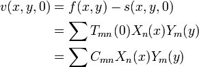
$\begin{align} v(x,y,0)&=f(x,y)-s(x,y,0) \\ &=\sum T_{mn}(0)X_n(x)Y_m(y) \\ &=\sum C_{mn}X_n(x)Y_m(y) \end{align}$

The Fourier coefficients can be solved using the inner product definition:

$C_{mn}=\frac{\int\limits_0^L \int\limits_0^M \left [ f(x,y)-s(x,y,0) \right ] X_n(x)Y_m(y) dy dx}{\int\limits_0^L X_n^2(x) dx \int\limits_0^M Y_m^2(y) dy}$

We have all the necessary information about the variable portion of the function.

Step 4: Combine Solutions

We now have solved for the "steady-state" and "variable" portions, so we just add them together to get the complete solution to the 2-D heat equation.

This article is issued from Wikiversity - version of the Thursday, December 30, 2010. The text is available under the Creative Commons Attribution/Share Alike but additional terms may apply for the media files.