Fourier transforms

The Fourier Transform represents a function $s \left( t \right)$ as a "linear combination" of complex sinusoids at different frequencies $\omega\,$ . Fourier proposed that a function may be written in terms of a sum of complex sine and cosine functions with weighted amplitudes.

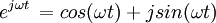
In Euler notation the complex exponential may be represented as:

$e^{j\omega t}\, = cos(\omega t) + j sin(\omega t)$

Thus, the definition of a Fourier transform is usually represented in complex exponential notation.

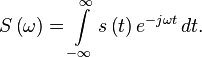
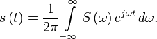
The Fourier transform of s(t) is defined by $S \left( \omega \right) = \int\limits_{-\infty}^\infty s\left( t\right) e^{-j\omega t}\,dt.$

Under appropriate conditions original function can be recovered by:

$s \left( t \right) = \frac{1}{2\pi} \int\limits_{-\infty}^\infty S\left( \omega\right) e^{j\omega t}\,d\omega.$

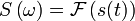
The function $S \left( \omega \right)$ is the Fourier transform of $s \left( t \right)$ . This is often denoted with the operator $\mathcal{F}$ , in the case above, $S \left( \omega \right) = \mathcal{F} \left(s ( t) \right)$

The function $s \left( t \right)$ must satisfy the Dirichlet conditions in order for $s \left( t \right)$ for the integral defining Fourier transform to converge.

Forward Fourier Transform(FT)/Anaysis Equation

$S \left( \omega \right) = \int\limits_{-\infty}^\infty s\left( t\right) e^{-j\omega t}\,dt.$

Inverse Fourier Transform(IFT)/Synthesis Equation

$s \left( t \right) = \frac{1}{2\pi} \int\limits_{-\infty}^\infty S\left( \omega\right) e^{j\omega t}\,d\omega.$

Relation to the Laplace Transform

In fact, the Fourier Transform can be viewed as a special case of the bilateral Laplace Transform. If the complex Laplace variable s were written as $s = \sigma + j \omega \,$ , then the Fourier transform is just the bilateral Laplace transform evaluated at $\sigma = 0 \,$ . This justification is not mathematically rigorous, but for most applications in engineering the correspondence holds.

Properties

×	Time Function	Fourier Transform	Property
1	$z(t)=x(t) \pm \ y(t)$	$Z(\omega)=X(\omega) \pm \ Y(\omega)$	Linearity
2	$Z(t)$	$2\pi z(-\omega)$	Duality
3	$c\, x(t)$ , c = constant	$c\, X(\omega)$	Scalar Multiplication
4	$\frac {dx(t)}{dt}$	$j \omega\,X(\omega)$	Differentiation in time domain
5	$\int\limits_{-x}^{t} x(\tau)d \tau$	$\frac {X(\omega)}{j \omega}$ , if $\int\limits_{-\infty}^{\infty} x(t)\,dt = 0$	Integration in Time domain
6	$t\,x(t)$	$j\,\frac {dX(\omega)}{d \omega}$	Differentiation in Frequency Domain
7	$x(-\,t)$	$X(-\,\omega)$	Time reversal
8	$x(a\,t)$	$\frac{1}{\left \| a \right \|}X\left( \frac {\omega}{a} \right )$	Time Scaling
9	$x(t\,-\,a)$	$e^{-\,j \omega\,a}\,X(\omega)$	Time shifting
10	$x(t) \cos {\omega_0\,t}$	$\frac{1}{2}\left [ X(\omega\,+\,\omega_0)\,+\,X(\omega\,-\,\omega_0) \right ]$	Modulation
11	$x(t) \sin {\omega_0\,t}$	$\frac{1}{2j}\left [ X(\omega\,-\,\omega_0)\,-\,X(\omega\,+\,\omega_0) \right ]$	Modulation
12	$e^{-\,a\,t}x(t)$	$X(\omega\,+\,a)$	Frequency shifting
13	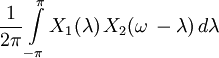$x_1(t)\times\,x_2(t)$	$\frac{1}{2 \pi}\int\limits_{- \pi}^{\pi}X_1(\lambda)\,X_2(\omega\,-\lambda)\,d\lambda$	Convolution

This article is issued from Wikiversity - version of the Tuesday, May 13, 2014. The text is available under the Creative Commons Attribution/Share Alike but additional terms may apply for the media files.