Energy methods in elasticity

Energy Methods/Variational Principles

Examples:

Principle of Virtual Work.
Principle of Minimum Potential Energy.
Principle of Minimum Complementary Energy.
Hu-Washizu Variational Principle.
Hellinger-Reissner Variational Principle.

Why ?

Powerful way of approaching problems in linear elasticity.
Can be used to derive the governing equations and boundary conditions for special classes of problems.
Used as the basis of approximate solutions of elasticity problem, e.g., finite element method.
Can be used to obtain rigorous bounds on the stiffness of elastic structures/solids.

Some definitions from Variational Calculus

Functional

A functional is basically a function of some other functions. Let $u(x)$ be the displacement. Then the local strain energy density $U[u(x)]$ is a functional.

The Minimization Problem

Find $u(x)$ such that

U[u(x)] = \int_{x_0}^{x_1} F(x,u,u^{'}) dx

is a minimum.

Variation

Suppose

U[u(x) + \delta u(x)] \ge U[u(x)] ~\forall~ |\delta u(x)| < h ~\text{and}~ x \in (x_0, x_1)

and equality holds only when $\delta u(x) = 0\,$ . Then $\delta u\,$ is the variation of $u\,$ .

Necessary Condition : Euler Equation

A necessary condition that $u(x)$ minimizes $U[u(x)]$ is that the Euler equation

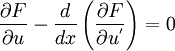
\frac{\partial F}{\partial u} - \frac{d}{dx}\left(\frac{\partial F}{\partial u^{'}} \right) = 0

is satisfied and

\left.\frac{\partial F }{\partial u^{'}} \right|_{x_0} = 0 ~~\text{or,}~~ \eta(x_0) = 0

and,

\left.\frac{\partial F}{\partial u^{'}} \right|_{x_1} = 0 ~~\text{or,}~~ \eta(x_1) = 0

where

\delta u(x) = \epsilon \eta(x)

and $\epsilon$ is small and $\eta(x)$ is arbitrary.

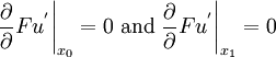
Imposed BCs

The imposed BCs are the conditions

\eta(x_0) = 0~\text{and}~ \eta(x_1) = 0

These are automatically satisfied.

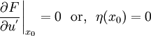
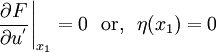
Natural BCs

The natural BCs are the conditions

\left.\frac{\partial }{\partial} {F}{u^{'}}\right|_{x_0} = 0 ~\text{and} \left.\frac{\partial }{\partial} {F}{u^{'}}\right|_{x_1} = 0

Stationary Functions

Any $u(x)$ that satisfies the necessary conditions make the functional $U[u(x)]$ stationary and is said to be a stationary function of the functional.

Taking Variations

Suppose that $U$ is a functional with

U[u(x)] = \int_{x_0}^{x_1} F(x,u,u^{'}) dx

Suppose that $\delta u$ is a small variation of $u$ that satisfies

\left|\delta u(x)\right| \ll 1 ~;~~ \left|\delta u^{'}(x)\right| \ll 1 ~\forall~ x \in (x_0,x_1)

Then the variation of $F$ is

\delta F = F(x,u+\delta u,u^{'}+\delta u^{'}) -F(x,u,u^{'})\,

or,

\delta F = \frac{\partial F}{\partial u}~\delta u + \frac{\partial F }{\partial u^{'}}~ \delta u^{'}

The variation of $U$ is

\delta U = \int_{x_0}^{x_1} \delta F dx

or,

\delta U = \left.\frac{\partial F}{\partial u^{'}} ~ \delta u \right|_{x_0}^{x_1} + \int_{x_0}^{x_1} \left[ \frac{\partial F }{\partial u} ~\delta u - \frac{d}{dx}\left(\frac{\partial F }{\partial u^{'}} \right)\delta u\right] dx

Assuming that $\delta U = 0\,$ is a necessary condition to minimize $U[u(x)]\,$ , we get the same necessary conditions as before.

Lagrange Multipliers

If there are additional constraints on minimization, we usually use Lagrange Multipliers.

Suppose the additional constraint is that $x + u + u^{'} = C$ . Then, we define a function,

\tilde{F(x,u,u^{'},\lambda)} = F(x,u,u^{'}) - \lambda\left[x + u + u^{'} - C\right]

where $\lambda$ is the Lagrange multiplier.

Then,

\frac{\partial \tilde{F} }{\partial \lambda} = 0

Then, the values that minimize the function subject to the given constraint are given by the equations

\frac{\partial \tilde{F}}{\partial \lambda} = 0 ~~;~~ \frac{\partial \tilde{F}}{\partial u } = 0 ~~;~~ \frac{\partial \tilde{F}}{\partial u^{'}} = 0

More on Strain Energy Density

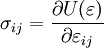
Recall that the strain energy density is defined as

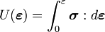
U(\boldsymbol{\varepsilon}) = \int_0^{\varepsilon} \boldsymbol{\sigma}:d\boldsymbol{\varepsilon}

If the strain energy density is path independent, then it acts as a potential for stress, i.e.,

\sigma_{ij} = \frac{\partial U(\varepsilon) }{\partial \varepsilon_{ij}}

For adiabatic processes, $U$ is equal to the change in internal energy per unit volume.

For isothermal processes, $U$ is equal to the Helmholtz free energy per unit volume.

The natural state of a body is defined as the state in which the body is in stable thermal equilibrium with no external loads and zero stress and strain.

When we apply energy methods in linear elasticity, we implicitly assume that a body returns to its natural state after loads are removed. This implies that the Gibb's condition is satisfied :

U(\boldsymbol{\varepsilon}) \ge 0 ~~\text{with}~~ U(\boldsymbol{\varepsilon}) = 0 ~~\text{iff}~~ \boldsymbol{\varepsilon} = 0

The Principle of Virtual Work

This principle is used in the derivation of several minimization principles and states that:

If $\sigma^{(1)}_{ij}$ is a state of stress satisfying equilibrium

\boldsymbol{\nabla}\bullet{\boldsymbol{\sigma}^{(1)}} + \mathbf{f}^{(1)} = 0~~\text{on}~ B

and the traction boundary condition

\widehat{\mathbf{n}}{}\bullet\boldsymbol{\sigma}^{(1)} = \mathbf{t}^{(1)} ~~\text{on}~ \partial B

Also, if $u^{(2)}$ is a displacement field on $B$ such that the strain field $\varepsilon^{(2)}_{ij}$ is given by

\varepsilon^{(2)} = \frac{1}{2}\left(\boldsymbol{\nabla}u^{(2)} + (\boldsymbol{\nabla}u^{(2)})^T\right)

then

\int_{B} f_i^{(1)} u_i^{(2)}~ dV + \int_{\partial B} t_i^{(1)} u_i^{(2)}~ dA = \int_{B} \sigma_{ij}^{(1)} \varepsilon_{ij}^{(2)}~ dV

The converse also holds - and is usually more interesting because it gives us a different way of thinking about equilibrium.

Example

If there are jump discontinuities in a body, then what does equilibrium imply ?

Suppose that $\boldsymbol{\sigma}$ has a jump discontinuity across a body along the surface $S$ with normal $\hat{\mathbf{m}}$ because the materials on the two sides are different.

We define the equilibrium state to be one that satisfies the principle of virtual work for all displacement fields.

Now, if the spin tensor is zero, then

\sigma_{ij}^{(1)} \varepsilon_{ij}^{(2)} = (\sigma_{ij}^{(1)} u_i^{(2)})_{,j} - \sigma_{ij,j}^{(1)} u_i^{(2)}

If we use the above, and apply the divergence theorem to the virtual work equation we get

\int_{B} \left(\sigma^{(1)}_{ji,j} + f_i^{(1)} \right) u_i^{(2)}~ dV + \int_{\partial B} \left(t_i^{(1)} - \sigma_{ij}^{(1)} n_j\right) u_i^{(2)}~ dA = 0

For the stress jump to satisfy this equation, we must have

\int_{B} \left(\sigma^{(1)}_{ji,j} + f_i^{(1)} \right) u_i^{(2)}~ dV + \int_{\partial B} \left(t_i^{(1)} - \sigma_{ij}^{(1)} n_j\right) u_i^{(2)}~ dA + \int_S (\sigma_{ij}^{+} m_j^{+} - \sigma_{ij}^{-} m_j^{-}) u_i^{(2)} dS = 0

Hence, equilibrium is satisfied when

\sigma_{ij}^{+} m_j^{+} - \sigma_{ij}^{-} m_j^{-} = 0~~\text{on}~~ S

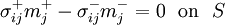
which means that even though a jump can exist in the stresses, the tractions have to be continuous across the discontinuity.

Energy as a Functional

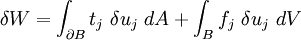
The work done by external forces on a body $B$ can be represented as a functional

W[\mathbf{u}] = \int_{\partial B} \left(\int_0^{\mathbf{u}} \mathbf{t}\bullet d\mathbf{u}\right) dA + \int_B \left(\int_0^{\mathbf{u}} \mathbf{f}\bullet d\mathbf{u}\right) dV

Taking the variation of $W$ , we get

\delta W = \int_{\partial B}\frac{\partial }{\partial \mathbf{u}} \left[ \left(\int_0^{\mathbf{u}} \mathbf{t}\bullet d\mathbf{u}\right)\right] dA + \int_B \frac{\partial }{\partial \mathbf{u}} \left[ \left(\int_0^{\mathbf{u}} \mathbf{f}\bullet d\mathbf{u}\right)\right] dV

In index notation,

\delta W = \int_{\partial B}\frac{\partial }{\partial u_j} \left[ \left(\int_0^{\mathbf{u}} t_i~du_i\right)\right]\delta u_j ~ dA + \int_B \frac{\partial }{\partial u_j} \left[ \left(\int_0^{\mathbf{u}} f_i~du_i\right)\right]\delta u_j ~ dV

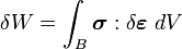
Noting that the external forces and body forces are not functions of $\mathbf{u}$ , the above equation reduces to

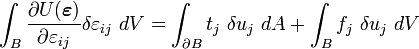
\delta W = \int_{\partial B} t_j~\delta u_j ~ dA + \int_Bf_j~ \delta u_j ~ dV

The above expression is called the external virtual work.

If we apply the principle of virtual work, with

\mathbf{t} = \mathbf{t}^{(1)} ~;~~ \mathbf{f} = \mathbf{f}^{(1)} ~;~~ \boldsymbol{\sigma} = \boldsymbol{\sigma}^{(1)} ~;~~ \delta\mathbf{u} = \mathbf{u}^{(2)} ~;~~ \delta\boldsymbol{\varepsilon} = \boldsymbol{\varepsilon}^{(2)}

we get

\delta W = \int_B \boldsymbol{\sigma} : \delta\boldsymbol{\varepsilon}~dV

or,

\delta W = \int_B \frac{\partial U(\boldsymbol{\varepsilon})}{\partial \varepsilon_{ij}} \delta\varepsilon_{ij}~dV

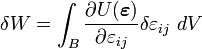
This is the expression for the internal virtual work.

Thus, another form of the principle of virtual work is

\int_B \frac{\partial U(\boldsymbol{\varepsilon})}{\partial \varepsilon_{ij}} \delta\varepsilon_{ij}~dV = \int_{\partial B} t_j~\delta u_j ~ dA + \int_Bf_j~ \delta u_j ~ dV

Doing the reverse operation, it can be shown that

W[\boldsymbol{\varepsilon}(\mathbf{x})] = \int_R U(\boldsymbol{\varepsilon})~dV

which relates the strain energy density ( $U$ ) to the functional $W$ that represents the work done by external forces.

Energy Minimization Principles

Developed and explored by Green (1839), Haughton(1849), Kirchhoff (1850), Love (1906), Trefftz (1928) and others.

The Principle of Stationary Potential Energy

This principle states that:

Among all possible kinematically admissible displacement fields
the potential energy functional is rendered stationary
by only those that are actual displacement fields.

The Principle of Minimum Potential Energy

This principle states that

If the prescribed traction and body force fields are independent of the deformation
then the actual displacement field makes the potential energy functional an absolute minimum.

Kinematically Admissible Displacement Fields

Consider a body $B$ with a boundary $\partial B$ with an applied body force field $\tilde{\mathbf{f}}$ .

Suppose that displacement BCs $\mathbf{u} = \tilde{\mathbf{u}}$ are prescribed on the part of the boundary $\partial B^u$ .

Suppose also that traction BCs $\widehat{\mathbf{n}}{}\bullet\boldsymbol{\sigma} = \tilde{\mathbf{t}}$ are applied on the portion of the boundary $\partial B^t$ .

A displacement field $(\mathbf{v})$ is kinematically admissible if

$\mathbf{v}$ satisfies the displacement boundary conditions $\mathbf{v} = \tilde{\mathbf{u}}$ on $\partial B^u$ .
$\mathbf{v}$ is continuously differentiable, i.e., $\mathbf{v} \in C^3(\mathbb{R})$ and $|\boldsymbol{\nabla}{\mathbf{v}}| << 1$ .

Potential Energy Functional

The potential energy functional associated with the kinematically admissible displacement field $\mathbf{v}$ is defined as

\Pi[\mathbf{v},\boldsymbol{\varepsilon},\boldsymbol{\sigma}] = \int_B U(\boldsymbol{\varepsilon})~dV - \int_B \tilde{\mathbf{f}}\bullet\mathbf{v}~dV - \int_{\partial B^t} \tilde{\mathbf{t}}\bullet\mathbf{v}~dA

or,

\Pi[\mathbf{v}] = \frac{1}{2}\int_B \boldsymbol{\nabla}{\mathbf{v}}:\mathbf{C}:\boldsymbol{\nabla}{\mathbf{v}}~dV - \int_B \tilde{\mathbf{f}}\bullet\mathbf{v}~dV - \int_{\partial B^t} \tilde{\mathbf{t}}\bullet\mathbf{v}~dA

In index notation,

\Pi[\mathbf{v}] = \frac{1}{2}\int_B C_{ijkl}~v_{k,l}~v_{i,j}~dV - \int_B \tilde{f}_i~v_i~dV - \int_{\partial B^t} \tilde{t}_i~v_i~dA

Stationary Points and Minimum of the Potential Energy Functional

What do we mean when we say that we "render the potential energy functional stationary" or "minimum"? Note that the potential energy is a functional of a vector field.

Suppose that the actual displacement field (one that satisfies equilibrium, compatibility and the boundary conditions) is $\mathbf{u}$ .

Let $\mathbf{v}$ be a kinematically admissible variation of $\mathbf{u}$ , i.e.,

\mathbf{v} = \mathbf{u} + k~\delta\mathbf{u}

where $k$ is a constant.

Then $\delta\mathbf{u}$ must be a displacement field that is continuously differentiable and satisfies the boundary conditions

\delta\mathbf{u} = 0 ~~\text{on}~~ \partial B^u

The potential energy functional for $\mathbf{v}$ is

\begin{align} \Pi[\mathbf{u} + k~\delta\mathbf{u}] = & \frac{1}{2}\int_B \boldsymbol{\nabla}{(\mathbf{u} + k~\delta\mathbf{u})}:\mathbf{C}: \boldsymbol{\nabla}{(\mathbf{u}+k~\delta\mathbf{u})}~dV \\ &- \int_B \tilde{\mathbf{f}}\bullet(\mathbf{u}+k~\delta\mathbf{u})~dV - \int_{\partial B^t} \tilde{\mathbf{t}}\bullet(\mathbf{u}+k~\delta\mathbf{u})~dA \end{align}

In index notation,

\begin{align} \Pi[\mathbf{u} + k~\delta\mathbf{u}] = & \frac{1}{2}\int_B C_{ijkl}(u_{i,j}+k~\delta u_{i,j}) (u_{k,l}+k~\delta u_{k,l})~dV \\ &- \int_B \tilde{f}_i(u_i+k~\delta u_i)~dV - \int_{\partial B^t} \tilde{t}_i(u_i+k~\delta u_i)~dA \end{align}

Expanding and rearranging,

\begin{align} \Pi[\mathbf{u} + k~\delta\mathbf{u}] = & \frac{1}{2}\int_B C_{ijkl}~u_{i,j}~u_{k,l}~dV - \int_B \tilde{f}_i~u_i~dV - \int_{\partial B^t} \tilde{t}_i~u_i~dA \\ & + k\left[\frac{1}{2}\int_B C_{ijkl}~u_{i,j}~\delta u_{k,l}~dV + \frac{1}{2}\int_B C_{ijkl}~\delta u_{i,j}~u_{k,l}~dV \right]\text{(1)} \qquad \\ & - k\left[\int_B \tilde{f}_i~\delta u_i~dV - \int_{\partial B^t} \tilde{t}_i~\delta u_i~dA\right] \\ & + \frac{k^2}{2}\int_B C_{ijkl}~\delta u_{i,j}~\delta u_{k,l}~dV \end{align}

Using the symmetry of the stiffness tensor, we can simplify the above expression and write it it terms of variations of $\Pi$ . Thus,

\Pi[\mathbf{u} + k~\delta\mathbf{u}] = \Pi[\mathbf{u}] + k~\delta\Pi[\mathbf{u},\delta\mathbf{u}] + \frac{1}{2} k^2~\delta^2\Pi(\mathbf{u},\delta\mathbf{u})

You can check that the first and second variations of $\Pi$ turn out to be equal to the expanded terms in equation (1).

Stationary Point

\delta\Pi(\mathbf{u},\delta\mathbf{u}) = 0

for all admissible variations $\delta\mathbf{u}$ , then $\mathbf{u}$ is a { stationary point} of the functional $\Pi$ .

Minimum

\delta^2\Pi(\mathbf{u},\delta\mathbf{u}) > 0

for all admissible variations $\delta\mathbf{u}$ , then $\mathbf{u}$ is makes the functional $\Pi$ a minimum.

Observations on Uniqueness and Existence of Solutions

The potential energy functional is a global minimum if and only if the displacement field satisfies traction BCs, equilibrium and the displacement BCs.
Thus, if the potential energy functional actually has a global mininum, then a solution exists and must be unique.
Displacement boundary value problems do not face the problem of rigid body motions. Therefore, a global minimum always exists for such problems and is unique.
Traction boundary value problems may not have unique solutions, nor might solutions always exist unless the external loads are in static equilibrium.

Example: Approximate Solutions of Torsion Problems

Suppose that we have a cylindrical body of length $L$ and an arbitrary cross-section that is subject to equal and opposite torques at the two ends. The displacement field is given by

u_1 = -\alpha x_2 x_3 ~;~~ u_2 = \alpha x_1 x_3 ~;~~ u_3 = \alpha \psi(x_1,x_2)

The traction-free boundary conditions on the lateral surfaces can be given as

\widehat{\mathbf{n}}{}\bullet\boldsymbol{\sigma} = 0

The torque BC at the ends can be replaced with displacement BCs

\text{on}~ x_3 = 0~;~~ ~~~~ u_1 = u_2 = 0 ~,~~ u_3 = \alpha\psi(x_1,x_2)

and

\text{on}~ x_3 = L~;~~ ~~~~ u_1 = -\alpha L x_2 ~,~~ u_2 = \alpha L x_1 ~,~~ u_3 = \alpha\psi(x_1,x_2)

Thus, we change the problem from a purely traction boundary value problem to one in which the twist per unit length ( $\alpha$ ) is prescribed instead of the applied torque ( $T$ ).

The modified problem is one with zero body force and zero tractions. Therefore, the potential energy functional reduces to

\Pi[\mathbf{v},\boldsymbol{\varepsilon},\boldsymbol{\sigma}] = \int_B U(\boldsymbol{\varepsilon})~dV

The stresses and strains for the torsion problem are given by

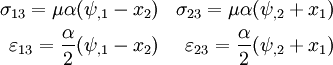
\begin{align} \sigma_{13} = \mu\alpha(\psi_{,1}-x_2) & & \sigma_{23} = \mu\alpha(\psi_{,2}+x_1) \\ \varepsilon_{13} = \frac{\alpha}{2}(\psi_{,1}-x_2) &&\varepsilon_{23} = \frac{\alpha}{2}(\psi_{,2}+x_1) \end{align}

Therefore, the internal energy is

U(\boldsymbol{\varepsilon}) = \frac{1}{2}\sigma_{ij}\varepsilon_{ij} = \frac{1}{2} \mu\alpha^2 \left[(\psi_{,1} - x_2)^2 + (\psi_{,2} + x_1)^2\right]

The potential energy per unit length ( $\bar{\Pi}$ ) is

\bar{\Pi}[\psi(x_1,x_2)] = \frac{1}{2} \mu\alpha^2 \int_{\mathcal{S}} \left[(\psi_{,1} - x_2)^2 + (\psi_{,2} + x_1)^2\right] dA

According to the principle of minimum potential energy, the actual warping function is the one that makes $\bar{\Pi}$ an absolute minimum.

Suppose we are given a warping function of the form

\psi = A x_1^2 + B x_1 x_2 + C x_2^2

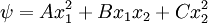
Then, the potential energy per unit length is

\begin{align} \bar{\Pi}[\psi(x_1,x_2)] = \frac{1}{2} \mu\alpha^2 &\left[ \int_{\mathcal{S}} \left[4A^2 + (B+1)^2\right] x_1^2~dA + \int_{\mathcal{S}} \left[4C^2 + (B-1)^2\right] x_2^2~dA +\right. \\ &\left.\int_{\mathcal{S}} 4\left[A(B-1) + C(B+1)\right] x_1~x_2~dA\right] \end{align}

If $x_1$ and $x_2$ are the principal axes of inertia, then we have

I_1 = \int_{\mathcal{S}} x_1^2~dA ~;~~ I_2 = \int_{\mathcal{S}} x_2^2~dA ~;~~ I_{12} = \int_{\mathcal{S}} x_1~x_2~dA = 0

Hence,

\begin{align} \bar{\Pi}[\psi(x_1,x_2)] = & \frac{1}{2} \mu\alpha^2 \left[ \left[4A^2 + (B+1)^2\right] I_1 + \left[4C^2 + (B-1)^2\right] I_2 \right] \end{align}

The stationary points of the potential energy functional are given by

\begin{align} \frac{\partial \bar{\Pi}}{\partial A} & = 4\mu\alpha^2~I_2~A = 0 \\ \frac{\partial \bar{\Pi}}{\partial B} & = \mu\alpha^2\left[(B+1)I_2+(B-1)I_1\right] = 0 \\ \frac{\partial \bar{\Pi}}{\partial C} & = 4\mu\alpha^2~I_2~A = 0 \end{align}

Thus, we have,

A = 0 ~;~~ B = \frac{I_1-I_2}{I_1+I_2} ~;~~ C = 0 \,

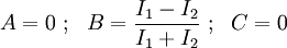
Thus the best approximation to the warping function is

\psi =\frac{I_1-I_2}{I_1+I_2} x_1 x_2 \,

The above technique is called the Rayleigh-Ritz method.

An important observation that should be made at this stage is about the approximate nature of the solution.

For cross-sections in which $I_1 = I_2\,$ , (e.g., circular or square sections) the best approximation for $\psi$ is $\psi = 0$ . This gives us the exact result for circular cross-sections.

However, for square cross-sections we have an error of nearly 20%.

Energy methods in elasticity

Energy Methods/Variational Principles

Some definitions from Variational Calculus

Functional

The Minimization Problem

Variation

Necessary Condition : Euler Equation

Imposed BCs

Natural BCs

Stationary Functions

Taking Variations

Lagrange Multipliers

More on Strain Energy Density

The Principle of Virtual Work

Example

Energy as a Functional

Energy Minimization Principles

The Principle of Stationary Potential Energy

The Principle of Minimum Potential Energy

Kinematically Admissible Displacement Fields

Potential Energy Functional

Stationary Points and Minimum of the Potential Energy Functional

Stationary Point

Minimum

Observations on Uniqueness and Existence of Solutions

Example: Approximate Solutions of Torsion Problems

Related Content