Electric Circuit Analysis/Mesh Analysis

Lesson Review 5 & 6:

What you need to remember from Kirchhoff's Voltage & Current Law .

• Remember what was learned in Passive sign convention, You can go back and revise Lesson 1.

• Kirchhoff's Voltage Law

• Kirchhoff's Current Law

This part of the course onwards will collaborate with the Mathematics Department extensively. Mathematical Theory will be kept minimal as mathematical tools are only used here as a means to an end. Links to relevant Mathematical theories will be supplied to assit the student.

Lesson Review 7:

What you need to remember from Nodal analysis. If you ever feel lost, do not be shy to go back to the previous lesson & go through it again. You can learn by repitition.

• Use KCL at super nodes to formulate circuit equations.
• Create matrix from circuit equations.
• Solve for Unknown Node Voltages using Cramer's Rule.

Lesson 8: Preview

This Lesson is about Mesh Analysis. The student/User is expected to understand the following at the end of the lesson.

• Use KVL at meshes or loops to formulate circuit equations.
• Create matrix from circuit equations.
• Solve for Unknown Mesh Currents using Cramer's Rule.

Part 1: Pre-reading Material

The student is advised to read the following resources from the Mathematics department:

• College Algebra
• Linear algebra

Part 2: Mesh Analysis

Let's start off with some useful definitions:

• Branch:

This is a circuit element(s) that connect two nodes.

• Loop:

This a closed path in a circuit. A set of these loops are used to create constraint equations.

• Mesh:

A loop passing though at least one branch.

Basic rule: The sum of Voltages arround any loop must be Zero.( From KVL in Lecture 5).

Part 3

The following is a general procedure for using Mesh or Loop Analysis method to solve electric circuit problems. The aim of this algorithm is to develop a matrix system from equations found by applying KVL arround Loops or Meshes in an electric circuit. Cramer's rule is then used to solve the unkown Mesh Currents.

Once the Mesh Currents are solved, normal circuit analysis methods ( Ohm's law; Voltage and Current Divider principles etc... ) can then be used to find whatever circuit entity.

Remember to consult previous lessons if you are not confident in using normal circuit analysis techniques that will be used in this lesson.

Manual Mesh/Loop Analysis Algorithm:

1.) Choose a conventional current flow.

2.) Identify and Number loops or meshes. ( Usually 2 or 3 meshes/ loops )

3.) Apply KVL to identified meshes/loops and formulate ciruit equations.

4.) Create Matrix system from KVL equations obtained.

5.) Solve Matrix for unknown Mesh Currents by using Cramer's rule ( it is simpler although you can still use gaussian method as well )

6.) Used solved Mesh Currents to solve for the desired circuit entity.

The above algorithm is very basic and usefull for 2 x 2 and 3 x 3 size matrices. Generally as the number of loops or meshes increase and the size of the matrix exceeds 3 x 3, numerical methods ( Beyond scope of this course ) are employed with the aid of computers to solve such circuit networks.

Generally speaking, Mesh Analysis is shorter than Nodal Analysis although not always preffered.Let's try an example to illustrate the above Mesh/Loop analysis algorithm.

Part 4 : Example

Figure 8.1: Example 1

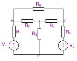
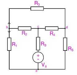
Consider Figure 8.1 with the following Parameters:

Find current through using Mesh Analysis method.
Solution:

Figure 8.2: Currents in loops

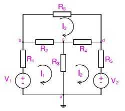
This is the same example we solved in Exercise 7.

We can see that there are three closed paths (loops) where we can apply KVL in, Loop 1, 2 and 3 as shown in figure 8.2

We can now apply KVL arround the loops remembering Passive Convention when defining Currents and voltages.

KVL arround abca loop:

Therefore

............(1)

Part 5 : Example (Continued)

KVL arround acda loop:

Therefore

   ...............   (2)

KVL arround bdcb loop:

Therefore

   ...............   (3)

Now we can create a matrix with the above equations as follows:

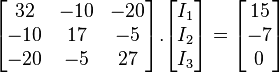
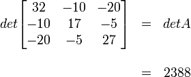
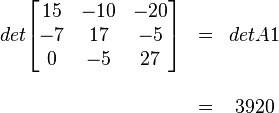
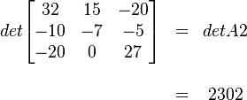
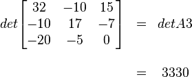
Part 6 : Example (Continued)

The following matrix is the above with values substituted:

?

Now that we have arranged equations 1; 2 & 3 into a matrix we need to get Determinants of the General matrix, and Determinants of alterations of the general matrix as follows:

Solving determinants of:

• Matrix A  : General matrix A from KVL equations

• Matrix A1 : Genral Matrix A with Column 1 substituted by .

• Matrix A2 : Genral Matrix A with Column 2 substituted by .

• Matrix A3 : Genral Matrix A with Column 3 substituted by .

As follows:

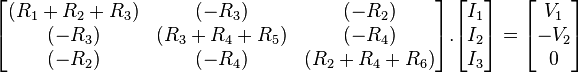
Part 7: Example (Continued)

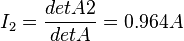
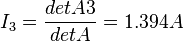
Part 8: Example (Continued)

Now we can use the solved determinants to arrive at solutions for Mesh Currents as follows:

1.

2.

3.

Now we can solve for the current through as follows:

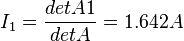
The answer is as we expected it to be, flows in the direction of . As expected, mesh analysis and nodal analysis gave equivalent answers.

Part 9: Exercise 8

Figure 8.3: Exercise

Consider Figure 8.3 with the following Parameters:

Find current through using Mesh Analysis method.

• Answers to Exercise 8

Part 10:

Further Reading Links:

• w:Mesh analysis

• Mesh-Currents Analysis Web Application

Refferences:

• Add refference here!

Completion List

Once you finish your Exercises you can post your score here! To post your score just e-mail your course co-ordinator your name and score *Click Here.

• 1. …
  2. …
  3. …