Econometrics

Econometrics 1

This course is concerned with theory and application of linear regression methods, including an examination of the classical regression model and the statistical properties of the estimator. The effect of violations of the classical assumptions are considered, and appropriate estimation methods are introduced. This course is the first of a two-course sequence. At course completion, a successful student will:

understand the statistical foundations of the classical regression model.
be able to explain the properties of the least-squares estimator and related test statistics.
be able to apply these methods to data and interpret the results.

Introduction and Review

Random variables

How do we handle random processes? We can define a random variable as a measurable function defined on a probability space. Bievens(2004)

See set theory. Kolmorgorov gives us the axioms of probability.

Firstly, the probability of some outcome, A, is greater than or equal to zero, $P(A)\ge0$ for A contained in the probability space S $A\in S$ .
Secondly, the probability over the sample space is equal to one, $P(S) = 1 \,$ .

Thirdly, the probability of A and B is equal to the probability of A plus the probability of B, if A and B are disjoint and contained in the sample space S $P(A+B)=P(A)+P(B); A\cap B=\oslash; A,B \in S$ .

For example, in a coin toss, the probability space is heads and tails. If x is a function over the probability space, we can say that x(heads) equals one and x(tails) equals zero. So the probability that x is one equals the probability of heads, and the probability that x is zero equals the probability of tails, and they are disjoint probabilities. So if the probability of heads is Ph, the probability of tails is 1-Ph. (Note that this example does not assume that you have a fair coin, though you could.)

Review of Matrices

positive semidefinite (PSD), positive definite (PD), quadratic forms, symettric, idempotent, diagonal, block diagonal,

Matix derivatives

The Probability Distribution Function is 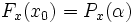$F_x(x_0) =P_x(\alpha)\,$ where $\alpha = {x|x\le x_0}$

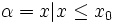
II. Fundamentals of Regression Analysis

Linear regression

By having a set of ys, assumed to be dependent on a set of xs, we solve for some constant $\beta \,$ . (Where k is the number of observations, and n is the number of predictor or independent variables, y is a kx1 vector and x is a kxn matrix multiplied by an nx1 vector $\beta\,$ which relates y and x.)

$y = x\beta + \epsilon\,$

To solve for $\beta\,$ , which will give us an expected value of $\beta\,$ that we will call beta hat $\hat\beta\,$ we use this linear operation:

$\hat\beta=(x'x)^{-1}x'y\,$

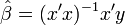
This can be derived from OLS, ordinary least squares, which minimizes the squared residuals. Since $y = x\beta + \epsilon\,$ , then $\epsilon = y - x\beta$ . The residuals are then the estimated errors $e$ , found from the estimated model: $e = y - x \hat\beta$ The squared residuals are then 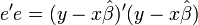$e'e = (y - x \hat\beta)'( y - x \hat\beta)$ . By deriving this expression with respect to $\hat\beta$ and solving for $\hat\beta$ gives the OLS estimator.

Then $x\hat\beta = \hat y$ or x times beta hat equals y hat, where y hat is our expected value for y given x and our calculated value of beta, beta hat.

Now the difference between the predicted values of y and the actual values of y are given by: $y-x\hat\beta=y-\hat y = e$ where $e\,$ is residual values, sometimes called error.

Matrix algebra,

Properties of Ordinary Least Squares (OLS estimator beta hat is unbiased for beta, and the Covariance Matrix for beta hat is $\sigma ^2 (x'x)^{-1}\,$ ), Classical Normal, The Information Matrix, Chi Square Distribution, The relationship between e and epsilon, The Maximum Likelihood Estimator of the variance is biased, Distribution of the variance under normality,

regression, principles of estimation and testing, stationary time series models, limited dependent variable models, longitudinal (panel) data models, generalized methods of moments, instrumental variable models, non-stationarity, stochastic trends, co-integration,

Errors in functional form specification

Omission of relevant explanatory variables

Inclusion of irrelevant explanatory variables

Nonlinear Regression Functions

Squared explanatory variables

Cubed explanatory variables

Multicollinearity

Rarely is perfect multicollinearity a problem, but multicollinearity, linear relationships between explanatory variables, often is. Multicollinearity causes an increase in the variance of ß estimations, which in turn decreases the probability of rejecting the null hypotheses that such ßs are insignificant.

Resources

Recommended texts

Davidson and MacKinnon "Econometric Theory and Methods"

DeGroot and Schervish "Probability and Statistics" 3rd edition

A review of matrix algebra is recommended. In econometrics, it is necessary to work with very large sets of data. In order to manipulate the data and follow the discussion, you must be familiar with matrices.

Wikibook Econometric Theory

This article is issued from Wikiversity - version of the Tuesday, September 18, 2012. The text is available under the Creative Commons Attribution/Share Alike but additional terms may apply for the media files.