Cubic Spline Interpolation
Cubic spline interpolation is a special case for Spline interpolation that is used very often to avoid the problem of Runge's phenomenon. This method gives an interpolating polynomial that is smoother and has smaller error than some other interpolating polynomials such as Lagrange polynomial and Newton polynomial.
Definition
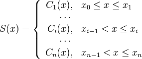
Given a set of n + 1 data points (xi,yi) where no two xi are the same and  , the spline S(x) is a function satisfying:
-
![S(x)\in C^2[a,b]](../I/m/cebbac110e4b8a675ade6038a34282a3.png) ;
; - On each subinterval
![[x_{i-1},x_{i}], S(x)](../I/m/c927a6cce067b14bcd52021e4ed24d13.png) is a polynomial of degree 3, where
is a polynomial of degree 3, where 
-
 for all
Let us assume that
where each  is a cubic function, .
Boundary Conditions
To determine this cubic spline S(x), we need to determine  for each i by:
-
 and
and  ,
, -
 ,
, 
-
 ,
,
We can see that there are  conditions, but we need to determine
  coefficients, so usually we add two boundary conditions to solve this problem.
There are three types of common boundary conditions:
I. First derivatives at the endpoints are known:
 .
.
The special case  is called clamped boundary conditions.
II. Second derivatives at the endpoints are known:
 .
.
The special case  is called natural or simple boundary conditions.
III. When the exact function f(x) is a periodic function with period  , S(x) is a periodic function with period too. Thus
 .
.
The spline functions S(x) satisfying this type of boundary condition are called periodic splines.
Methods
There are several methods that can be used to find the spline function S(x) according to its corresponding conditions. Since there are 4n coefficients to determine with 4n conditions, we can easily plug the values we know into the 4n conditions and then solve the system of equations. Note that all the equations are linear with respect to the coefficients, so this is workable and computer can do it quite well.
The algorithm given in w:Spline interpolation is also a method by solving the system of equations to obtain the cubic function in the symmetrical form.
The other method used quite often is w:Cubic Hermite spline, this gives us the spline in w:Hermite form.
Here, we discuss another method using second derivatives  to find the expression for spline S(x).
Let  ,
,  ,
,  and
and  . Note that
  's are unknown (except for type II boundary condition,
  are given).
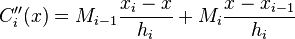
Since each  is a cubic polynomial,
  is linear.
By w:Lagrange interpolation, we can interpolate each on ![[x_{i-1},x_i]](../I/m/cd4ecc36c89db79c632a849e2e8a2adc.png) since
since  and
and 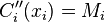 , the Lagrange form of this interpolating polynomial is:
 for
for ![x\in [x_{i-1},x_i]](../I/m/3c25e3f88aaf76551622fd2c2be6c9d7.png) .
.
Integrating the above equation twice and using the condition that
and to determine the constants of integration, we have
-
![C_i(x)=M_{i-1}\frac{(x_i-x)^3}{6h_i}+M_i\frac{(x-x_{i-1})^3}{6h_i}+(y_{i-1}-\frac{M_{i-1}h_i^2}{6})\frac{x_i-x}{h_i}+(y_{i}-\frac{M_{i}h_i^2}{6})\frac{x-x_{i-1}}{h_i}\quad\text{for}\quad x\in [x_{i-1},x_i].](../I/m/542b05f3064c6d37e57acca2b9c3546b.png)
(1 )
This expression gives us the cubic spline S(x) if  can be determined.
For  when
when ![x\in [x_{i},x_{i+1}],](../I/m/143c4c23a6bf96f33ca3adf8d1b3b60b.png) , we can calculate that
, we can calculate that

Therefore, 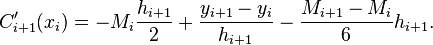
Similarly, when ![x\in [x_{i-1},x_{i}],](../I/m/27ccb6bceed21914dbaf2792f8c2becc.png) , we can shift the index to obtain
, we can shift the index to obtain
-

(2 )
Thus, 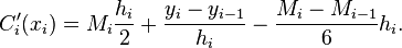
Since 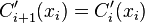 , we can derive
-

(3 )
where
-
![\mu_i=\frac{h_i}{h_{i}+h_{i+1}},\quad \lambda_i=1-\mu_i=\frac{h_{i+1}}{h_{i}+h_{i+1}},\quad\text{and}\quad d_i=6 f[x_{i-1},x_i,x_{i+1}]\,](../I/m/527ca5177980d6ed4ac524e4aa3cca25.png)
(4 )
and ![f[x_{i-1},x_i,x_{i+1}]](../I/m/d0f6197db79f081b433607027856bf73.png) is a divided difference.
is a divided difference.
According to different boundary conditions, we can solve the system of equations above to obtain the values of 's.
I. For type I boundary condition, we are given  and
and 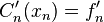 . According to equation (2
), we can obtain
. According to equation (2
), we can obtain

![\Rightarrow f'_0=-M_{0}\frac{h_1}{2}+f[x_0,x_1]-\frac{M_{1}-M_{0}}{6}h_{1}](../I/m/ca0b423fa743dc1178ddd561bc8c8c99.png)
-
![\Rightarrow 2M_{0}+M_{1}= \frac{6}{h_1}(f[x_0,x_1]-f'_0)=6f[x_0,x_0,x_1]](../I/m/0e631d7e924fd544247fc5ce9968f53d.png) .
.(5.1 )
-
Similarly, simplifying

we will have
-
![M_{n-1}+2M_{n}= \frac{6}{h_n}(f'_n-f[x_{n-1},x_n])=6f[x_{n-1},x_n,x_{n}]](../I/m/cdf749a947ed86421066d7a42ffc278a.png) .
.(5.2 )
-
Therefore, let ![\lambda_0=\mu_n=1, d_0=6f[x_0,x_0,x_1]](../I/m/45fc9ded86b986380d81faf696eacdb7.png) and
and ![d_n=6f[x_{n-1},x_n,x_n]](../I/m/3e68bd75433b9a26064a515b21f79d3c.png) , combine (3
), (5.1
) and (5.2
) together, so
the system of equations that we need to solve is
, combine (3
), (5.1
) and (5.2
) together, so
the system of equations that we need to solve is
-
![\left[\begin{array}{ccccccc}
2 & \lambda_0 & & & & & \\
\mu_1 & 2 & \lambda_1 & & & & \\
& \ddots & \ddots & \ddots & & &\\
& & \ddots & \ddots & \ddots & & \\
& & & \ddots & \ddots & \ddots & \\
& & & &\mu_{n-1} & 2 & \lambda_{n-1}\\
& & & & & \mu_n & 2
\end{array} \right]
\left[\begin{array}{c}
M_0 \\
M_1 \\
\vdots\\
\vdots\\
\vdots\\
M_{n-1}\\
M_n\end{array} \right]=
\left[\begin{array}{c}
d_0 \\
d_1 \\
\vdots\\
\vdots\\
\vdots\\
d_{n-1}\\
d_n\end{array} \right].](../I/m/24c99d92bfb2b4cefe92b3d40ba0f2ac.png)
(6 )
-
II. For type II boundary condition, we are given
-
 and
and 
(7 )
-
directly, so let  ,
,  , and
, and  , and we need to solve the system of equations in the same form as (6
).
, and we need to solve the system of equations in the same form as (6
).
Example
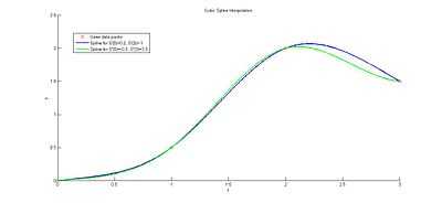
For points (0,0), (1,0.5), (2,2) and (3,1.5), find the interpolating cubic spline  satisfying
  and
and  .
.
Solution:
We can easily see that  for
for  so
so  and
and 
Also, since this is the type I boundary condition problem, we can calculate that
![f[x_0,x_1,x_0]=f[x_0,x_0,x_1]=(f[x_1,x_0]-f[x_0,x_0])/(x_1-x_0)=\left(\frac{0.5-0}{1-0}-0.2\right)/1=0.3;](../I/m/d5ea6910207cc872435aa24991a97e66.png)
![f[x_0,x_1,x_2]=f[x_0,x_1,x_2]=(f[x_2,x_1]-f[x_1,x_0])/(x_2-x_0)=\left(\frac{2-0.5}{1-0}-\frac{0.5-0}{1-0}\right)/2=0.5;](../I/m/b1be327ea5f21884fcc12733986f0587.png)
![f[x_1,x_2,x_3]=f[x_1,x_2,x_3]=(f[x_3,x_2]-f[x_2,x_1])/(x_3-x_1)=\left(\frac{1.5-2}{1-0}-\frac{2-0.5}{1-0}\right)/2=-1;](../I/m/14dea4f917bfcdf749340b168c3babb8.png) and
and![f[x_3,x_2,x_3]=f[x_2,x_3,x_3]=(f[x_3,x_3]-f[x_2,x_3])/(x_3-x_2)=\left(-1-\frac{1.5-2}{1-0}\right)/1=-\frac{1}{2}.](../I/m/877fed443f61b2316f3b50120fdf8b1d.png)
Therefore, plug into the system of equations, we have
![\left[\begin{array}{cccc}
2 & 1 & & \\
1/2 & 2 & 1/2 & \\
& 1/2 & 2 & 1/2\\
& & 1 & 1/2\end{array} \right]
\left[\begin{array}{c}
M_0 \\
M_1 \\
M_2\\
M_3\end{array} \right]=
\left[\begin{array}{c}
6\times 0.3 \\
6\times 0.5 \\
6\times (-1)\\
6\times (-1/2)\end{array} \right].](../I/m/843185c13ce5bc6bb4de3da323929b92.png)
The solution is  and
and 
Therefore, by the general expression of the solution, we have
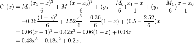
Similarly,
 and
and
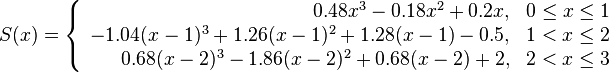
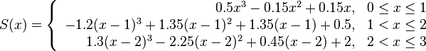
Thus the cubic spline is
Exercise
Therefore, we can construct the system of equations:
Solution:
![\left[\begin{array}{cccc}
2 & 0 & & \\
1/2 & 2 & 1/2 & \\
& 1/2 & 2 & 1/2\\
& & 0 & 2\end{array} \right]
\left[\begin{array}{c}
M_0 \\
M_1 \\
M_2\\
M_3\end{array} \right]=
\left[\begin{array}{c}
-0.6 \\
3 \\
-6\\
6.6\end{array} \right].](../I/m/1bf301dd058bcdec40590da341ccf1fc.png)
Since  and
and  , we can find the solution:
 and
and  .
.
Plug these into the general expression for cubic spline and simplify, we can obtain
You can see the difference of the two cubic splines in Figure 1.
References
Polynomial and Spline Interpolation, http://www.math.ohiou.edu/courses/math3600/lecture19.pdf
数值分析,李庆扬,王能超,易大易,2001. ISBN 7-302-04561-5 (Numerical Analysis, Qinyang Li, Nengchao Wang, Dayi yi.)