Coordinate transformations

Vector Transformation in Two Dimensions

In three dimensions, the vector transformation rule is written as

v^{'}_i = l_{ij} v_j

where $\textstyle l_{ij} = \mathbf{e}^{'}_i\bullet\mathbf{e}_j = \cos(\mathbf{e}^{'}_i,\mathbf{e}_j)$ .

In two dimensions, this transformation rule is the familiar

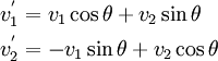
\begin{align} v^{'}_1 & = v_1 \cos\theta + v_2 \sin\theta \\ v^{'}_2 & = -v_1 \sin\theta + v_2 \cos\theta \\ \end{align}

In matrix form,

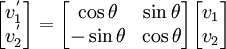
\begin{bmatrix} v^{'}_1 \\ v^{'}_2 \end{bmatrix} = \begin{bmatrix} \cos\theta & \sin\theta \\ -\sin\theta & \cos\theta \\ \end{bmatrix} \begin{bmatrix} v_1 \\ v_2 \end{bmatrix}

Since we are using sines, the direction of measurement of $\textstyle \theta$ is required. In this case, it is measured counterclockwise.

Tensor Transformation in Two Dimensions

In three dimensions, the second-order tensor transformation rule is written as

T^{'}_{ij} = l_{ip} l_{jq} T_{pq}

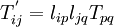
where $\textstyle l_{ij} = \mathbf{e}^{'}_i\bullet\mathbf{e}_j = \cos(\mathbf{e}^{'}_i,\mathbf{e}_j)$ .

The Cauchy stress $\textstyle \boldsymbol{\sigma}$ is a symmetric second-order tensor. In two dimensions, the transformation rule for stress is the written as

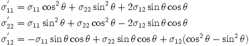
\begin{align} \sigma^{'}_{11} & = \sigma_{11} \cos^2\theta + \sigma_{22} \sin^2\theta + 2 \sigma_{12} \sin\theta\cos\theta \\ \sigma^{'}_{22} & = \sigma_{11} \sin^2\theta + \sigma_{22} \cos^2\theta - 2 \sigma_{12} \sin\theta\cos\theta \\ \sigma^{'}_{12} & = -\sigma_{11} \sin\theta\cos\theta + \sigma_{22} \sin\theta\cos\theta + \sigma_{12}(\cos^2\theta-\sin^2\theta) \end{align}

In matrix form,

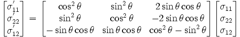
\begin{bmatrix} \sigma^{'}_{11} \\ \sigma^{'}_{22} \\ \sigma^{'}_{12} \end{bmatrix} = \begin{bmatrix} \cos^2\theta & \sin^2\theta & 2 \sin\theta\cos\theta \\ \sin^2\theta & \cos^2\theta & - 2\sin\theta\cos\theta \\ -\sin\theta\cos\theta & \sin\theta\cos\theta & \cos^2\theta-\sin^2\theta \end{bmatrix} \begin{bmatrix} \sigma_{11} \\ \sigma_{22} \\ \sigma_{12} \end{bmatrix}

Since we are using sines, the direction of measurement of $\textstyle \theta$ is required. In this case, it is measured counterclockwise.

Tensor Transformation in two Dimensions, the intrinsic approach

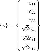
Let construct an orthonormal basis of the second order tensor projected in the first order tensor

E_{1}=e_1 \otimes e_1

E_{2}=e_2 \otimes e_2

E_{3}=e_3 \otimes e_3

E_{4}=\frac{1}{\sqrt{2}}(e_2 \otimes e_3 + e_3 \otimes e_2)

E_{5}=\frac{1}{\sqrt{2}}( e_3 \otimes e_1 + e_1 \otimes e_3)

E_{6}=\frac{1}{\sqrt{2}}( e_1 \otimes e_2 + e_2 \otimes e_1)

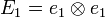
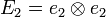
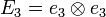
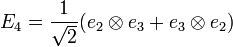
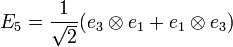
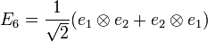
The stress and strain tensors are now defined by :

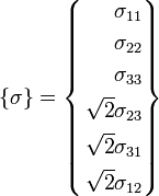
\left \{\sigma \right \} = \left \{ \begin{align} \sigma_{11} \\ \sigma_{22} \\ \sigma_{33} \\ \sqrt{2}\sigma_{23} \\ \sqrt{2}\sigma_{31} \\ \sqrt{2}\sigma_{12} \\ \end{align} \right \}

and

\left \{\varepsilon \right \} = \left \{ \begin{align} \varepsilon_{11} \\ \varepsilon_{22} \\ \varepsilon_{33} \\ \sqrt{2}\varepsilon_{23} \\ \sqrt{2}\varepsilon_{31} \\ \sqrt{2}\varepsilon_{12} \\ \end{align} \right \}

Then once constructs the bound matrix in the orthonormal base $E_{i} \otimes E_{j}$

\left [ \hat{R}(\theta) \right ]= \left [ \begin{matrix} R_{11}^2 & R_{12}^2 & R_{13}^2 & \sqrt{2}R_{12}R_{13} & \sqrt{2}R_{11}R_{13} & \sqrt{2}R_{11}R_{12}\\ R_{21}^2 & R_{22}^2 & R_{23}^2 & \sqrt{2}R_{22}R_{23} & \sqrt{2}R_{21}R_{23} & \sqrt{2}R_{22}R_{21}\\ R_{31}^2 & R_{32}^2 & R_{33}^2 & \sqrt{2}R_{33}R_{32} & \sqrt{2}R_{33}R_{31} & \sqrt{2}R_{31}R_{32}\\ \sqrt{2}R_{21}R_{31} & \sqrt{2}R_{22}R_{32} & \sqrt{2}R_{23}R_{33} & R_{22}R_{33}+R_{23}R_{32} & R_{21}R_{33}+R_{31}R_{23} & R_{21}R_{32}+R_{31}R_{22}\\ \sqrt{2}R_{11}R_{31} & \sqrt{2}R_{12}R_{32} & \sqrt{2}R_{13}R_{33} & R_{12}R_{33}+R_{32}R_{13} & R_{11}R_{33}+R_{13}R_{31} & R_{11}R_{32}+R_{31}R_{12}\\ \sqrt{2}R_{11}R_{21} & \sqrt{2}R_{12}R_{22} & \sqrt{2}R_{13}R_{23} & R_{12}R_{23}+R_{22}R_{13} & R_{11}R_{23}+R_{21}R_{13} & R_{11}R_{22}+R_{21}R_{12}\\ \end{matrix} \right ]

with

$\left [ R(\theta) \right ]$ the rotation matrix in $e_{i} \otimes e_{j}$ base.

Example

\left [ R(\theta) \right ]= \left [ \begin{matrix} 1 & 0 & 0 \\ 0 & cos \theta & sin \theta \\ 0 & -sin \theta& cos \theta \end{matrix} \right ]

is the rotation along the axis $e_1$ in the : $e_i \otimes e_j$ base

The associated rotation in the $E_i \otimes E_j$ base is :

\left [ \hat{R}(\theta) \right ]= \left [ \begin{matrix} 1 & 0 & 0 & 0 & 0 & 0 \\ 0 & cos^2 \theta & sin^2 \theta & \sqrt{2} sin \theta cos \theta & 0 & 0 \\ 0 & sin^2 \theta & cos^2 \theta & -\sqrt{2} sin \theta cos \theta & 0 & 0 \\ 0 & - \sqrt{2} sin \theta cos \theta & \sqrt{2} sin \theta cos \theta & cos^2 \theta - sin^2 \theta & 0 & 0\\ 0 & 0 & 0 & 0 & cos \theta & -sin \theta \\ 0 & 0 & 0 & 0 & sin \theta & cos \theta \\ \end{matrix} \right ]

The rotation of a second order tensor is now defined by :

\left \{ \sigma(\theta) \right \} = {\left [ \hat{R}(\theta) \right ]}^T \left \{ \sigma \right \}

Four order tensor

The élasticity tensor 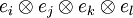$C_{ijkl}$ in the : $e_i \otimes e_j \otimes e_k \otimes e_l$ is defined in the : $E_i\otimes E_j$ by

\left [ \overline{C} \right ] = \left[\begin{align} C_{1111} & C_{1122} & C_{1133} & \sqrt{2}C_{1123} & \sqrt{2}C_{1131} & \sqrt{2}C_{1112} \\ C_{1122} & C_{2222} & C_{2233} & \sqrt{2}C_{2223} & \sqrt{2}C_{2231} & \sqrt{2}C_{2212} \\ C_{1133} & C_{2233} & C_{3333} & \sqrt{2}C_{3323} & \sqrt{2}C_{3331} & \sqrt{2}C_{3312} \\ \sqrt{2}C_{1123} & \sqrt{2}C_{2223} & \sqrt{2}C_{2333} & 2C_{2323} & 2C_{2331} & 2C_{2312} \\ \sqrt{2}C_{1131} & \sqrt{2}C_{2231} & \sqrt{2}C_{3331} & 2C_{2331} & 2C_{3131} & 2C_{3112} \\ \sqrt{2}C_{1112} & \sqrt{2}C_{2212} & \sqrt{2}C_{3312} & 2C_{2312} & 2C_{3112} & 2C_{1212} \end{align}\right]

and is rotated by:

{\left [ \overline{C} (\theta) \right ]}_g = {\left [ \hat{R}(\theta) \right ]}^T \left [ \overline{C} \right ]\left [ \hat{R}(\theta) \right ]