Coordinate systems/Derivation of formulas

< Coordinate systems

The purpose of this resource is to carefully examine the Wikipedia article Del in cylindrical and spherical coordinates for accuracy.

The identities are reproduced below, and contributors are encouraged to either:

Verify the identity and place its reference using a five em padding after the equation: {{pad|5em}}verified<ref>reference</ref>
Contribute to Wikiveristy by linking the title to a discussion and/or proof. Just click the redlink and start the page.

If you just came in from Wikipedia, the rules about treating each other with respect and obeying copyright laws remain more or less the same as on Wikipedia, but the definition of what constitutes an acceptable article is a lot looser. Here we call them "resources". Welcome to the wacky world of Wikiversity, where anything goes.

Transformations between coordinates

w:Cartesian coordinates (x, y, z)
w:Cylindrical coordinates (ρ, ϕ, z)
w:Spherical coordinates (r, θ, ϕ)
w:Parabolic cylindrical coordinates (σ, τ, z)

Coordinate variable transformations*

*Asterisk indicates that the title is a link to more discussion

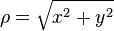
Cylindrical from Cartesian variable transformation

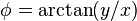$\rho = \sqrt{x^2+y^2}$ , $\phi = \arctan(y/x)$ , $z = z$ verified using mathworld^[1]

Cartesian from cylindrical variable transformation

$x = \rho\cos\phi$ , $y = \rho\sin\phi$ , $z = z$ verified using mathworld^[2]

Cartesian from spherical variable transformation

$x = r\sin\theta\cos\phi$ , $y = r\sin\theta\sin\phi$ , $z = r\cos\theta$ verified using mathworld^[3]

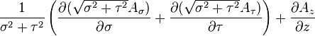
Cartesian from parabolic cylindrical variable transformation

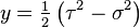$x = \sigma \tau$ , $y = \tfrac{1}{2} \left( \tau^{2} - \sigma^{2} \right)$ , $z = z$ --no reference

Spherical from Cartesian variable transformation

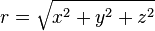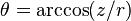$r = \sqrt{x^2+y^2+z^2}$ , $\theta = \arccos(z/r)$ , $\phi = \arctan(y/x)$ verified using mathworld^[4]

Spherical from cylindrical variable transformation

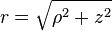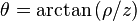$r = \sqrt{\rho^2 + z^2}$ , $\theta = \arctan{(\rho/z)}$ , $\phi = \phi$ no reference

Cylindrical from spherical variable transformation

$\rho = r\sin\theta$ , $\phi = \phi$ , $z = r\cos\theta$ no reference

Cylindrical from parabolic cylindrical variable transformation

$\rho\cos\phi = \sigma \tau$ , $\rho\sin\phi = \tfrac{1}{2} \left( \tau^{2} - \sigma^{2} \right)$ , $z = z$ no reference

Unit vectors

Cylindrical from Cartesian unit vectors

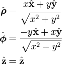$\begin{align} \hat{\boldsymbol\rho} &= \frac{ x \hat{\mathbf x} + y \hat{\mathbf y}}{\sqrt{x^2+y^2}} \\ \hat{\boldsymbol\phi} &= \frac{- y \hat{\mathbf x} + x \hat{\mathbf y}}{\sqrt{x^2+y^2}} \\ \hat{\mathbf z} &= \hat{\mathbf z} \end{align}$ Verified, see page linked in title

Cartesian from cylindrical unit vectors

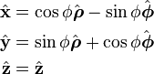$\begin{align} \hat{\mathbf x} &= \cos\phi\hat{\boldsymbol\rho} - \sin\phi\hat{\boldsymbol\phi} \\ \hat{\mathbf y} &= \sin\phi\hat{\boldsymbol\rho} + \cos\phi\hat{\boldsymbol\phi} \\ \hat{\mathbf z} &= \hat{\mathbf z} \end{align}$ Verified, see page linked in title

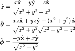
Cartesian from spherical unit vectors

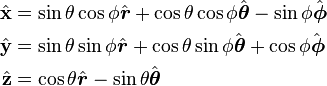$\begin{align} \hat{\mathbf x} &= \sin\theta\cos\phi\hat{\boldsymbol r} + \cos\theta\cos\phi\hat{\boldsymbol\theta}-\sin\phi\hat{\boldsymbol\phi} \\ \hat{\mathbf y} &= \sin\theta\sin\phi\hat{\boldsymbol r} + \cos\theta\sin\phi\hat{\boldsymbol\theta}+\cos\phi\hat{\boldsymbol\phi} \\ \hat{\mathbf z} &= \cos\theta \hat{\boldsymbol r} - \sin\theta \hat{\boldsymbol\theta} \end{align}$ Verified, see page linked in title

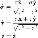
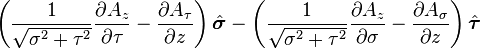
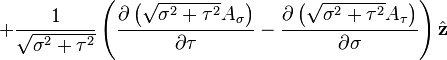
Parabolic cylindrical from Cartesian unit vectors

$\begin{align} \hat{\boldsymbol\sigma} &= \frac{\tau \hat{\mathbf x} - \sigma \hat{\mathbf y}}{\sqrt{\tau^2+\sigma^2}} \\ \hat{\boldsymbol\tau} &= \frac{\sigma \hat{\mathbf x} + \tau \hat{\mathbf y}}{\sqrt{\tau^2+\sigma^2}} \\ \hat{\mathbf z} &= \hat{\mathbf z} \end{align}$

Spherical from Cartesian unit vectors

$\begin{align} \hat{\mathbf r} &= \frac{x \hat{\mathbf x} + y \hat{\mathbf y} + z \hat{\mathbf z}}{\sqrt{x^2+y^2+z^2}} \\ \hat{\boldsymbol\theta} &= \frac{x z \hat{\mathbf x} + y z \hat{\mathbf y} - \left(x^2 + y^2\right) \hat{\mathbf z}}{\sqrt{x^2+y^2} \sqrt{x^2+y^2+z^2}} \\ \hat{\boldsymbol\phi} &= \frac{- y \hat{\mathbf x} + x \hat{\mathbf y}}{\sqrt{x^2+y^2}} \end{align}$ Verified, see page linked in title

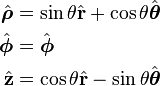
Spherical from cylindrical unit vectors

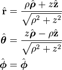
$\begin{align} \hat{\mathbf r} &= \frac{\rho \hat{\boldsymbol\rho} + z \hat{\mathbf z}}{\sqrt{\rho^2 +z^2}} \\ \hat{\boldsymbol\theta} &= \frac{ z \hat{\boldsymbol\rho} - \rho \hat{\mathbf z}}{\sqrt{\rho^2 +z^2}} \\ \hat{\boldsymbol\phi} &= \hat{\boldsymbol\phi} \end{align}$

Cylindrical from spherical unit vectors

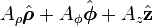
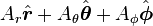
$\begin{align} \hat{\boldsymbol\rho} &= \sin\theta \hat{\mathbf r} + \cos\theta \hat{\boldsymbol\theta} \\ \hat{\boldsymbol\phi} &= \hat{\boldsymbol\phi} \\ \hat{\mathbf z} &= \cos\theta \hat{\mathbf r} - \sin\theta \hat{\boldsymbol\theta} \end{align}$

Vector and scalar fields

$\mathbf A$ is vector field and f is a scalar field. The vector field can be expressed as:

$A_x \hat{\mathbf x} + A_y \hat{\mathbf y} + A_z \hat{\mathbf z}$
$A_\rho \hat{\boldsymbol\rho} + A_\phi \hat{\boldsymbol\phi} + A_z \hat{\mathbf z}$
$A_r \hat{\boldsymbol r} + A_\theta \hat{\boldsymbol\theta} + A_\phi \hat{\boldsymbol\phi}$
$A_\sigma \hat{\boldsymbol\sigma} + A_\tau \hat{\boldsymbol\tau} + A_\phi \hat{\mathbf z}$

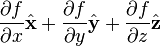
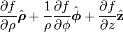
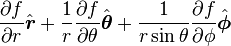
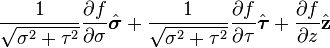
Gradient of a scalar field

$\nabla f$ is the w:gradient of a scaler field.

${\partial f \over \partial x}\hat{\mathbf x} + {\partial f \over \partial y}\hat{\mathbf y} + {\partial f \over \partial z}\hat{\mathbf z}$
${\partial f \over \partial \rho}\hat{\boldsymbol \rho} + {1 \over \rho}{\partial f \over \partial \phi}\hat{\boldsymbol \phi} + {\partial f \over \partial z}\hat{\mathbf z}$
${\partial f \over \partial r}\hat{\boldsymbol r} + {1 \over r}{\partial f \over \partial \theta}\hat{\boldsymbol \theta} + {1 \over r\sin\theta}{\partial f \over \partial \phi}\hat{\boldsymbol \phi}$
$\frac{1}{\sqrt{\sigma^{2} + \tau^{2}}} {\partial f \over \partial \sigma}\hat{\boldsymbol \sigma} + \frac{1}{\sqrt{\sigma^{2} + \tau^{2}}} {\partial f \over \partial \tau}\hat{\boldsymbol \tau} + {\partial f \over \partial z}\hat{\mathbf z}$

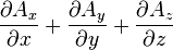
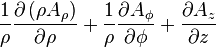
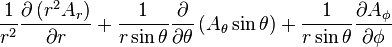
Divergence of a vector field*

$\nabla \cdot \mathbf{A}$ is the w:divergence of a vector field

${\partial A_x \over \partial x} + {\partial A_y \over \partial y} + {\partial A_z \over \partial z}$
${1 \over \rho}{\partial \left( \rho A_\rho \right) \over \partial \rho} + {1 \over \rho}{\partial A_\phi \over \partial \phi} + {\partial A_z \over \partial z}$
${1 \over r^2}{\partial \left( r^2 A_r \right) \over \partial r} + {1 \over r\sin\theta}{\partial \over \partial \theta} \left( A_\theta\sin\theta \right) + {1 \over r\sin\theta}{\partial A_\phi \over \partial \phi}$
$\frac{1}{\sigma^{2} + \tau^{2}}\left({\partial (\sqrt{\sigma^2+\tau^2} A_\sigma) \over \partial \sigma} + {\partial (\sqrt{\sigma^2+\tau^2} A_\tau) \over \partial \tau}\right) + {\partial A_z \over \partial z}$

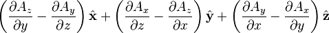
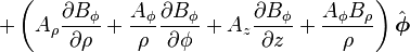
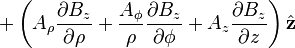
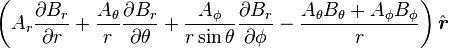
Curl of a vector field

$\nabla \times \mathbf{A}$ is the w:curl (mathematics) of A

$\left(\frac{\partial A_z}{\partial y} - \frac{\partial A_y}{\partial z}\right) \hat{\mathbf x} + \left(\frac{\partial A_x}{\partial z} - \frac{\partial A_z}{\partial x}\right) \hat{\mathbf y} + \left(\frac{\partial A_y}{\partial x} - \frac{\partial A_x}{\partial y}\right) \hat{\mathbf z}$
$\left( \frac{1}{\rho} \frac{\partial A_z}{\partial \phi} - \frac{\partial A_\phi}{\partial z} \right) \hat{\boldsymbol \rho} + \left( \frac{\partial A_\rho}{\partial z} - \frac{\partial A_z}{\partial \rho} \right) \hat{\boldsymbol \phi} + \frac{1}{\rho} \left( \frac{\partial \left(\rho A_\phi\right)}{\partial \rho} - \frac{\partial A_\rho}{\partial \phi} \right) \hat{\mathbf z}$
$\frac{1}{r\sin\theta} \left( \frac{\partial}{\partial \theta} \left(A_\phi\sin\theta \right) - \frac{\partial A_\theta}{\partial \phi} \right) \hat{\boldsymbol r} + \frac{1}{r} \left( \frac{1}{\sin\theta} \frac{\partial A_r}{\partial \phi} - \frac{\partial}{\partial r} \left( r A_\phi \right) \right) \hat{\boldsymbol \theta} + \frac{1}{r} \left( \frac{\partial}{\partial r} \left( r A_\theta \right) - \frac{\partial A_r}{\partial \theta} \right) \hat{\boldsymbol \phi}$
$\left( \frac{1}{\sqrt{\sigma^2 + \tau^2}} \frac{\partial A_z}{\partial \tau} - \frac{\partial A_\tau}{\partial z} \right) \hat{\boldsymbol \sigma} - \left( \frac{1}{\sqrt{\sigma^2 + \tau^2}} \frac{\partial A_z}{\partial \sigma} - \frac{\partial A_\sigma}{\partial z} \right) \hat{\boldsymbol \tau}$ $+ \frac{1}{\sqrt{\sigma^2 + \tau^2}} \left( \frac{\partial \left(\sqrt{\sigma^2 + \tau^2} A_\sigma \right)}{\partial \tau} - \frac{\partial \left(\sqrt{\sigma^2 + \tau^2} A_\tau \right)}{\partial \sigma} \right) \hat{\mathbf z}$

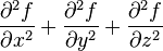
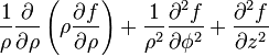
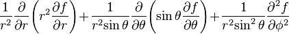
Laplacian of a scalar field

$\Delta f \equiv \nabla^2 f$ is the w:Laplace operator on a scalar field

${\partial^2 f \over \partial x^2} + {\partial^2 f \over \partial y^2} + {\partial^2 f \over \partial z^2}$
${1 \over \rho}{\partial \over \partial \rho}\left(\rho {\partial f \over \partial \rho}\right) + {1 \over \rho^2}{\partial^2 f \over \partial \phi^2} + {\partial^2 f \over \partial z^2}$
${1 \over r^2}{\partial \over \partial r}\!\left(r^2 {\partial f \over \partial r}\right) \!+\!{1 \over r^2\!\sin\theta}{\partial \over \partial \theta}\!\left(\sin\theta {\partial f \over \partial \theta}\right) \!+\!{1 \over r^2\!\sin^2\theta}{\partial^2 f \over \partial \phi^2}$
$\frac{1}{\sigma^{2} + \tau^{2}} \left( \frac{\partial^{2} f}{\partial \sigma^{2}} + \frac{\partial^{2} f}{\partial \tau^{2}} \right) + \frac{\partial^{2} f}{\partial z^{2}}$

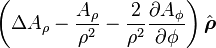
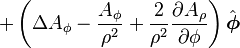
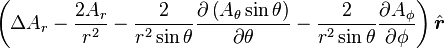
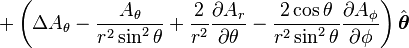
Laplacian of a vector field

$\Delta \mathbf{A} \equiv \nabla^2 \mathbf{A}$ is the w:Vector Laplacian of $\mathbf{A}$

$\Delta A_x \hat{\mathbf x} + \Delta A_y \hat{\mathbf y} + \Delta A_z \hat{\mathbf z}$
$\mathopen{}\left(\Delta A_\rho - \frac{A_\rho}{\rho^2} - \frac{2}{\rho^2} \frac{\partial A_\phi}{\partial \phi}\right)\mathclose{} \hat{\boldsymbol\rho}$ $+ \mathopen{}\left(\Delta A_\phi - \frac{A_\phi}{\rho^2} + \frac{2}{\rho^2} \frac{\partial A_\rho}{\partial \phi}\right)\mathclose{} \hat{\boldsymbol\phi}$ $+ \Delta A_z \hat{\mathbf z}$
$\left(\Delta A_r - \frac{2 A_r}{r^2} - \frac{2}{r^2\sin\theta} \frac{\partial \left(A_\theta \sin\theta\right)}{\partial\theta} - \frac{2}{r^2\sin\theta}{\frac{\partial A_\phi}{\partial \phi}}\right) \hat{\boldsymbol r}$ $+ \left(\Delta A_\theta - \frac{A_\theta}{r^2\sin^2\theta} + \frac{2}{r^2} \frac{\partial A_r}{\partial \theta} - \frac{2 \cos\theta}{r^2\sin^2\theta} \frac{\partial A_\phi}{\partial \phi}\right) \hat{\boldsymbol\theta}$ $+ \left(\Delta A_\phi - \frac{A_\phi}{r^2\sin^2\theta} + \frac{2}{r^2\sin\theta} \frac{\partial A_r}{\partial \phi} + \frac{2 \cos\theta}{r^2\sin^2\theta} \frac{\partial A_\theta}{\partial \phi}\right) \hat{\boldsymbol\phi}$

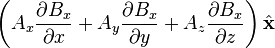
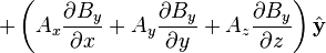
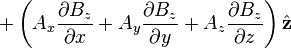
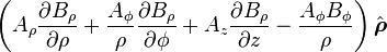
Material derivative of a vector field

$(\mathbf{A} \cdot \nabla) \mathbf{B}$ might be called the "convective derivative of B along A" (appropriate description if A' is a unit vector) ^[5]

$\left(A_x \frac{\partial B_x}{\partial x} + A_y \frac{\partial B_x}{\partial y} + A_z \frac{\partial B_x}{\partial z}\right) \hat{\mathbf{x}}$ $+ \left(A_x \frac{\partial B_y}{\partial x} + A_y \frac{\partial B_y}{\partial y} + A_z \frac{\partial B_y}{\partial z}\right) \hat{\mathbf{y}}$ $+ \left(A_x \frac{\partial B_z}{\partial x} + A_y \frac{\partial B_z}{\partial y} + A_z \frac{\partial B_z}{\partial z}\right) \hat{\mathbf{z}}$
$\left(A_\rho \frac{\partial B_\rho}{\partial \rho}+\frac{A_\phi}{\rho}\frac{\partial B_\rho}{\partial \phi}+A_z\frac{\partial B_\rho}{\partial z}-\frac{A_\phi B_\phi}{\rho}\right) \hat{\boldsymbol\rho}$ $+ \left(A_\rho \frac{\partial B_\phi}{\partial \rho} + \frac{A_\phi}{\rho}\frac{\partial B_\phi}{\partial \phi} + A_z\frac{\partial B_\phi}{\partial z} + \frac{A_\phi B_\rho}{\rho}\right) \hat{\boldsymbol\phi}$ $+ \left(A_\rho \frac{\partial B_z}{\partial \rho}+\frac{A_\phi}{\rho}\frac{\partial B_z}{\partial \phi}+A_z\frac{\partial B_z}{\partial z}\right) \hat{\mathbf z}$
$\left( A_r \frac{\partial B_r}{\partial r} + \frac{A_\theta}{r} \frac{\partial B_r}{\partial \theta} + \frac{A_\phi}{r\sin\theta} \frac{\partial B_r}{\partial \phi} - \frac{A_\theta B_\theta + A_\phi B_\phi}{r} \right) \hat{\boldsymbol r}$ $+ \left( A_r \frac{\partial B_\theta}{\partial r} + \frac{A_\theta}{r} \frac{\partial B_\theta}{\partial \theta} + \frac{A_\phi}{r\sin\theta} \frac{\partial B_\theta}{\partial \phi} + \frac{A_\theta B_r}{r} - \frac{A_\phi B_\phi\cot\theta}{r} \right) \hat{\boldsymbol\theta}$ $+ \left( A_r \frac{\partial B_\phi}{\partial r} + \frac{A_\theta}{r} \frac{\partial B_\phi}{\partial \theta} + \frac{A_\phi}{r\sin\theta} \frac{\partial B_\phi}{\partial \phi} + \frac{A_\phi B_r}{r} + \frac{A_\phi B_\theta \cot\theta}{r} \right) \hat{\boldsymbol\phi}$

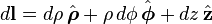
Differential displacement

$d\mathbf{l} = dx \, \hat{\mathbf x} + dy \, \hat{\mathbf y} + dz \, \hat{\mathbf z}$
$d\mathbf{l} = d\rho \, \hat{\boldsymbol \rho} + \rho \, d\phi \, \hat{\boldsymbol \phi} + dz \, \hat{\mathbf z}$
$d\mathbf{l} = dr \, \hat{\mathbf r} + r \, d\theta \, \hat{\boldsymbol \theta} + r \, \sin\theta \, d\phi \, \hat{\boldsymbol \phi}$
$d\mathbf{l} = \sqrt{\sigma^2 + \tau^2} \, d\sigma \, \hat{\boldsymbol \sigma} + \sqrt{\sigma^2 + \tau^2} \, d\tau \, \hat{\boldsymbol \tau} + dz \, \hat{\mathbf z}$

Differential normal areas

These vector differentials cannot be integrated for curved surfaces. Click the title above to see why.

Differential normal area $d \mathbf S$

$dy \, dz \hat{\mathbf x} + dx \, dz \hat{\mathbf y} + dx \, dy \hat{\mathbf z}$
$\rho \, d\phi \, dz \hat{\boldsymbol\rho} + d\rho \, dz \hat{\boldsymbol\phi} + \rho \, d\rho \, d\phi \hat{\mathbf z}$
$r^2 \sin\theta \, d\theta \, d\phi \hat{\mathbf r} + r \sin\theta \, dr \, d\phi \hat{\boldsymbol\theta} + r \, dr \, d\theta \hat{\boldsymbol\phi}$
$\sqrt{\sigma^2 + \tau^2} \, d\tau \, dz \hat{\boldsymbol\sigma} + \sqrt{\sigma^2 + \tau^2} \, d\sigma \, dz \hat{\boldsymbol\tau} + \left(\sigma^2 + \tau^2\right) \, d\sigma \, d\tau \hat{\mathbf z}$

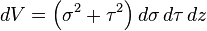
Differential volume

$dV=dx \, dy \, dz$ verified^[6]
$dV=\rho \, d\rho \, d\phi \, dz$ verified^[7]
$dV=r^2 \sin\theta \, dr \, d\theta \, d\phi$ verified^[8]
$dV=\left(\sigma^2 + \tau^2\right) d\sigma \, d\tau \, dz$

nabla's on nabla's

Non-trivial calculation rules:

$\operatorname{div} \, \operatorname{grad} f \equiv \nabla \cdot \nabla f = \nabla^2 f \equiv \Delta f$
$\operatorname{curl} \, \operatorname{grad} f \equiv \nabla \times \nabla f = \mathbf 0$
$\operatorname{div} \, \operatorname{curl} \mathbf{A} \equiv \nabla \cdot (\nabla \times \mathbf{A}) = 0$
$\operatorname{curl} \, \operatorname{curl} \mathbf{A} \equiv \nabla \times (\nabla \times \mathbf{A}) = \nabla (\nabla \cdot \mathbf{A}) - \nabla^2 \mathbf{A}$ (Lagrange's formula for del)
$\Delta (f g) = f \Delta g + 2 \nabla f \cdot \nabla g + g \Delta f$

References

↑ http://mathworld.wolfram.com/CylindricalCoordinates.html
↑ http://mathworld.wolfram.com/CylindricalCoordinates.html
↑ http://mathworld.wolfram.com/SphericalCoordinates.html
↑ http://mathworld.wolfram.com/SphericalCoordinates.html
↑
↑ James Stewart, Calculus: Concepts and Contexts, fourth edition, Brooks Cole 2005 pp. 884-5
↑ James Stewart, Calculus: Concepts and Contexts, fourth edition, Brooks Cole 2005 pp. 884-5
↑ James Stewart, Calculus: Concepts and Contexts, fourth edition, Brooks Cole 2005 pp. 884-5

^[1]

^[2]

↑ Weisstein, Eric W. "Convective Operator". Mathworld. Retrieved 23 March 2011.
↑ Huba J.D. (1994). "NRL Plasma Formulary revised". Office of Naval Research. Retrieved 11 June 2014.

Backup copy from Wikipedia

Copy or read but never change Original Copy from Wikipedia

This article is issued from Wikiversity - version of the Monday, August 11, 2014. The text is available under the Creative Commons Attribution/Share Alike but additional terms may apply for the media files.