Coordinate systems
This resource focuses on an introduction suitable for an introductory college physics course in electromagnetism.
We describe three different coordinate systems, known as Cartesian, cylindrical and spherical. The cylindrical system is closely related to polar coordinates.
See also Derivation of formulas
Cartesian Coordinates[1]
To the left: Illustration of a Cartesian coordinate plane. Four points are marked and labeled with their coordinates: (2, 3) in green, (−3, 1) in red, (−1.5, −2.5) in blue, and the origin (0, 0) in purple.
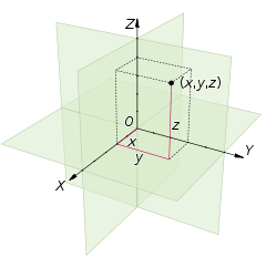
To the right: A three dimensional Cartesian coordinate system, with origin O and axis lines X, Y and Z, oriented as shown by the arrows. The tick marks on the axes are one length unit apart. The black dot shows the point with coordinates x = 2, y' = 3, and z = 4, or (2,3,4).
Line element in Cartesian coordinates
The distance between points  and
and  is
is

In other coordinate systems, it is best to focus on the distance between two points that are close together. For our purposes, it is best to replace the above formula with:
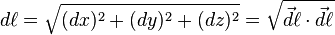
where,
 .
.
is known as a line element.
Line integral of a vector field in Cartesian coordinates
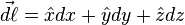
So far we have discussed the integral of a scalar field,  . An example of a scalar field is the temperature as a function of position (at any given time). Wind velocity as a function of position would be a vector field. In Cartesian coordinates it is easy to analyze a vector field as being equivalent to three scalar fields, one for each direction: Let
  (so that
Fx=f,
Fy=g,
and Fz=h). The line integral of the vector field from
(so that
Fx=f,
Fy=g,
and Fz=h). The line integral of the vector field from  to
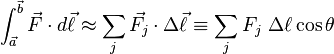
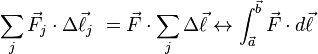
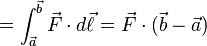
to  can now be defined as the limit of a Riemann sum:
Line integral of a uniform field over a straight path
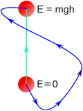
Line integrals are trivial if the vector field is uniform, meaning that the field does not depend on position. A well known example is the acceleration of gravity at Earth's surface, under the assumption that we may approximate the Earth as 'flat':  where g=9.8m/s2, and the 0 subscript reminds us that the field is a constant. Constant terms may be factored out of either a Riemann sum or an integral:
If
where g=9.8m/s2, and the 0 subscript reminds us that the field is a constant. Constant terms may be factored out of either a Riemann sum or an integral:
If  does not depend on position, then:

Note how the integral notation permits us to state the endpoint,  and starting point,
  , of the path. This can be evaluated to assume:
- See the Escher Waterfall to appreciate the technology that would be made possible if weight were not a conservative force.
Differential volume element in Cartesian coordinates
The Cartesian volume element is,

which easily permits a volume integral over a rectangular box. The integral of a function f=f(x,y,z) over the box is the triple integral, which is often informally written using a single integral, sign  .
.
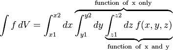
Note how the variable of integration (x or y or z) will disappear each time the integral is evaluated between the endpoints. This is a scalar integral if the function,  . In general, the limits may be functions, for example (z1,z2) may be functions of x and y, while (y1,y2) may be functions of x. Fortunately such complexity is not required in the volume integrals needed to understand electromagnetism.
Volume integral over a rectangular box
If none of the limits, (z1,z2) and (y1,y2), in the above integral are functions, then the integral is over a rectangular box. The most elementary example of such an integral occurs when  :
:

This is just the volume of the box.
Differential surface element in Cartesian coordinates
Surface integrals can also be viewed as the limit of a Riemann sum, but can be more difficult to construct than line or volume integrals unless the geometry is very simple. The differential element of surface area can either be a scalar,  , or the vector element,
  . Here,
  is normal to the surface.

At the moment of this writing a Wikipedia page states[2] that a surface element in Cartesian coordiantes is,

which is at best misleading.[3] In practice, one learns electromagnetism by doing very simple surface integrals where only one term is present.
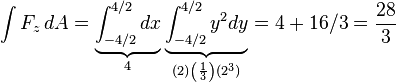
A surface integral over a square with its normal parallel to a Cartesian axis
The vector surface area element,
occupies rectangle parallel to the xy-plane. If the integral is of the form  , and the area is a square of length L centered at the origin, and occupying the plane, z=H, then:

In contrast to the one-dimensional integrals of a first-year calculus course, limits are not always used to define the region over which the field is integrated. Instead it is customary to state the integral,  , and then use words to describe the area (e.g. "where the integral is over a square with sides of length, L, centered at the origin and occupying the xy plane"). Very simply defined surface integrals can also be defined using limits. For example,

actually does describe a surface integral over a square with sides of length, L, that occupies the xy plane, and is centered at the origin. For example, if L=4, and
 ,
,
we have:
Polar coordinates
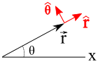
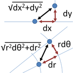
In the two-dimensional polar coordinate system, the displacement vector,  is specified by the distance to the origin,
  , and the angle,
  , measured with respect to the x-axis. The unit vectors (shown in red),
  and
and  are orthonormal, but change direction as the angle changes. It is evident from the two figures that:

![d\ell = \sqrt{ (dr)^2+r^2(d\theta)^2 }=
\left[ \left(\frac{dr}{d\tau}\right)^2 + r^2 \left(\frac{d\theta}{d\tau}\right)^2 \right]^{1/2}](../I/m/67cb05c00d583f2a97d530d28803eb07.png)

Cylindrical coordinates[4]
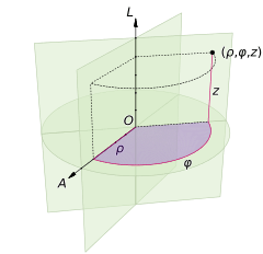
The cylindrical coordinate system specifies point positions by the symbols  , as shown in the figure. The coordinate
  can be positive or negative, while
  is always positive. Sometimes the Greek r, (called rho), is written in Latin form, , in order to avoid confusion with rho as charge density, and also in order to emphasize the close relationship between polar and cylindrical coordinates.
The line element is
The volume element is

The surface element in a surface of constant radius (a vertical cylinder) is

The surface element in a surface of constant azimuth  (a vertical half-plane) is

The surface element in a surface of constant height (a horizontal plane) is

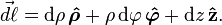
Spherical coordinates[5]


While three surface elements exist (one for each direction), the only one commonly used to introduce electrodynamics is in the radial direction:

Recall that the radian can be defined in terms of an arclength on a circle:  . By analogy, the solid angle can be defined through an area on a sphere:
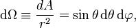
where dA is an area element taken on the surface of a sphere of radius, r, centered at the origin.
The volume element is spherical coordinates is:

Introductory discussions of electromagnetism often involve spherical symmetry, in which fields do not depend on the two directional coordinates (φ and θ). This permits integration over both variables:

We have just shown that the solid angle associated with a sphere is 4π steradians (just as the circle is associated with 2π radians).
Divergence, gradient and Laplacian (differential operators)
from https://en.wikipedia.org/w/index.php?title=Divergence&oldid=605214437
Cartesian coordinates
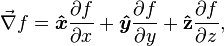
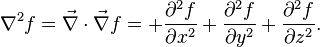
The del operator acting on a scalar field is the gradient of that field:
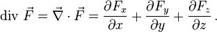
The divergence of a the vector field  is
is
The Laplacian  of a scalar field is
Cylindrical coordinates
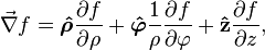
The del operator acting on a scalar field is the gradient of that field:
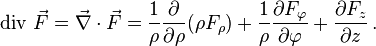
The divergence of a the vector field is
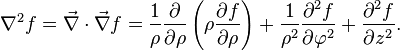
The Laplacian of a scalar field is
Advanced topics in vector integrals
The most well-known integrals of vector calculus are deliberately chosen to be simple because the intent is usually to depict important concepts in physics. This section describes moderately difficult geometries.
Line integral of scalar field
The most elementary line integral is along an axis. For example,
is the line integral of  from the point
  to
to  . A line an an arbitrary direction may be defined parametrically, e.g., by:

To define scalar line integral, we need to convert the vector path differential into a scalar by taking the magnitude. It is customary to label a differential in the vector using the symbol  instead of
  because the latter falsely hints at a change in radius, as we shall soon see:
where  is the vector magnitude. Writing the path differential
  as
as  would lead to great confusion when the (scalar) magnitude is taken because
  creates a conflict with the differential in radius if spherical coordinates are used:
  . The scalar line integral over a scalar field, is therefore:

is the line integral of from the point to .
If  , the three components of
  are the cosines that each coordinate axis (x-y-z) makes with . The most convenient way to express the differential line vector and scalar are:

![d\ell =\sqrt{dx^2+dy^2}=
\left[ \left(\frac{dx}{d\tau}\right)^2 + \left(\frac{dx}{d\tau}\right)^2 \right]^{1/2}d\tau](../I/m/c81e5efd548a064b9105c615e9795ac6.png)
Appendix: Teaching the vector
The "vector" is a nontrivial concept that arises even in Riemannian calculus where an n-dimensional space of variables is defined, and the concept of metric is used to generate vector and tensor fields, all without that fundamental sense of "direction" that students use to define "vector".
A students' introduction to coordinates starts with points on a two-dimensional x-y plane. There are a number of more or less equivalent way to label these points. We begin with the displacement vector:

This is essentially an ordered pair of variables that represent the real numbers x and y, and the formalism is easily extended to an arbitrary number of dimensions: :
One can define the displacement vector as an instruction to move a certain distance in a certain direction. In a Euclidean space, there is no difference between specifying a location (x,y) and an instruction to step from the origin in a certain direction to the point (x,y).
One advantage that vector notation offers is the ability to use symbols to represent a vector, and subscripts to represent the components:
- a=ax i + ay j and b=bx i + by j
This notation uses boldface instead of arrows and hats to distinguish between vectors and scalars. (In other words, a, and are different way to express the same thing.) The w:scalar (physics) or w:scalar (mathematics) is just a fancy word for "ordinary number". For example, ax and ay are scalars that form the two components of vector a. A famous use of different symbols to represent different vectors is F=ma, which says that the vector acceleration, a, multiplied the scalar, m, equals the net force, F (the latter being a vector because it has magnitude and direction).
Wikipedia links
- w:Vector calculus identities
- w:Surface integral
- Cartesian coordinates
- Polar coordinates
- Cylindrical cordinates
- w:Cylindrical coordinate system#Line and volume elements
- w:Spherical coordinate system#Integration and differentiation in spherical coordinates
- Unit vector (Wikipedia)
- w:standard basis (Wikipedia)
- w:Vector Calculus
other links
- ↑ from
- ↑ Quoting a misleading or false statement is unusual, but in this case serves to emphasize the need to not rely on Wikipedia whenever there are consequences to being wrong.
- ↑ (1)
 is not how the surface integral is usually set up. Nevertheless,
  , as shown above, is a vector area element. The usual way is to use a cross product and a surface defined in parametric form:
(2)
, as shown above, is a vector area element. The usual way is to use a cross product and a surface defined in parametric form:
(2) 
 We can now "force" (1) to occur with
(3)
We can now "force" (1) to occur with
(3)  In this context, writing (1) is putting the proverbial round peg into a square hole.
 - ↑ from https://en.wikipedia.org/w/index.php?title=Cylindrical_coordinate_system&oldid=606250748
- ↑ https://en.wikipedia.org/w/index.php?title=Spherical_coordinate_system&oldid=608581087