Continuum mechanics/Volume change and area change
< Continuum mechanicsVolume change
Consider an infinitesimal volume element in the reference configuration.
If a right-handed orthonormal basis in the reference configuration is
 then the vectors representing the edges of the
element are
then the vectors representing the edges of the
element are

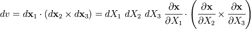
The volume of the element is given by

Upon deformation, these edges go to  where
where

or,

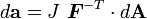
Therefore, the deformed volume is given by
Now,
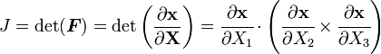
Hence,
|
|

Recall that from conservation of mass we have
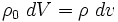
Therefore, an alternative form of the conservation of mass is
|
|

Distortional component of the deformation gradient
For many materials it is convenient to decompose the deformation gradient in a volumetric part and a distortional part. This is particularly useful when there is no volume change in the material when it deforms - for example in muscles, rubber tires, metal plasticity, etc.
Let us assume that the deformation gradient can be decomposed into a volumetric part and a distortional part, i.e,
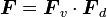
Then

Since there is no volume change due to the pure distortion, we have
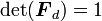
If 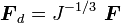 we have

Therefore the distortional component of the deformation gradient is given by
|
|
We can use this result to find the distortional components of various strain and deformation tensors. For example, the left Cauchy-Green deformation tensor is given by
If we define its distortional component as
we have
|
|
Area change - Nanson's formula
Nanson's formula is an important relation that can be used to go from areas in the current configuration to areas in the reference configuration and vice versa.
This formula states that
|
|
where  is an area of a region in the current configuration,
  is the same area in the reference configuration, and
  is the outward normal to the area element in the current configuration while
  is the outward normal in the reference configuration.
Proof:
To see how this formula is derived, we start with the oriented area elements in the reference and current configurations:
The reference and current volumes of an element are
where
.
Therefore,
or,
or,
So we get
or,