Continuum mechanics/Thermoelasticity
< Continuum mechanicsThermoelastic materials
A set of constitutive equations is required to close to system of balance laws. These are relations between appropriate kinematic quantities and stress measures that can be assigned a physical meaning.
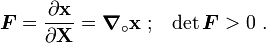
Deformation gradient as the strain measure
In thermoelasticity we assume that the fundamental kinematic quantity is the deformation gradient ( ) which is given by
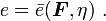
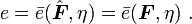
A thermoelastic material is one in which the internal energy ( ) is a function only of and the specific entropy (
 ), that is
For a thermoelastic material, we can show that the entropy inequality can be written as
|
|

At this stage, we make the following constitutive assumptions:
1) Like the internal energy, we assume that  and
and  are also functions only of and , i.e.,

2) The heat flux  satisfies the thermal conductivity inequality and if is independent of
  and
and  , we have

i.e., the thermal conductivity  is positive semidefinite.
Therefore, the entropy inequality may be written as
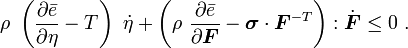
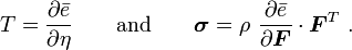
Since and are arbitrary, the entropy inequality will be satisfied if and only if

Therefore,
|
|
Given the above relations, the energy equation may expressed in terms of the specific entropy as
|
|

Effect of a rigid body rotation of the internal energy
If a thermoelastic body is subjected to a rigid body rotation  , then its internal energy should not change. After a rotation, the new deformation gradient (
 ) is given by
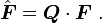
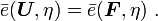
Since the internal energy does not change, we must have
Now, from the polar decomposition theorem,  where
where  is the orthogonal rotation tensor (i.e.,
  ) and
) and  is the symmetric right stretch tensor. Therefore,

We can choose any rotation . In particular, if we choose  , we have

Therefore,
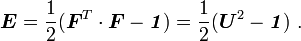
This means that the internal energy depends only on the stretch and not on the orientation of the body.
Other strain and stress measures
The internal energy depends on only through the stretch . A strain measure that reflects this fact and also vanishes in the reference configuration is the Green strain
|
|
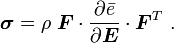
Recall that the Cauchy stress is given by
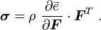
We can show that the Cauchy stress can be expressed in terms of the Green strain as
|
|
Also, recall that the first Piola-Kirchhoff stress tensor is defined as

Alternatively, we may use the nominal stress tensor
From the conservation of mass, we have  . Hence,
|
|
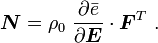
The first P-K stress and the nominal stress are unsymmetric. Also recall that we can define a symmetric stress measure with respect to the reference configuration called the second Piola-Kirchhoff stress tensor ( ):
):
|
|
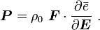
In terms of the derivatives of the internal energy, we have
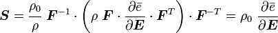
Therefore,
and
That is,
|
|

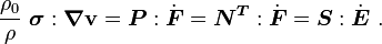
Stress Power
The stress power per unit volume is given by  . In terms of the stress measures in the reference configuration, we have
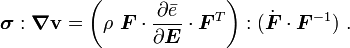
Using the identity  , we have
![\boldsymbol{\sigma}:\boldsymbol{\nabla}\mathbf{v} =
\left[
\left(\rho~\boldsymbol{F}\cdot\frac{\partial \bar{e}}{\partial \boldsymbol{E}}\cdot\boldsymbol{F}^T\right)\cdot\boldsymbol{F}^{-T}
\right] :\dot{\boldsymbol{F}}
= \rho~\left(\boldsymbol{F}\cdot\frac{\partial \bar{e}}{\partial \boldsymbol{E}}\right):\dot{\boldsymbol{F}}
= \cfrac{\rho}{\rho_0}~\boldsymbol{P}:\dot{\boldsymbol{F}}
= \cfrac{\rho}{\rho_0}~\boldsymbol{N}^T:\dot{\boldsymbol{F}}~.](../I/m/c1636b3a8db7ade0d938f906acb455d2.png)
We can alternatively express the stress power in terms of and  . Taking the material time derivative of
  we have
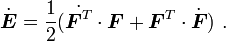
Therefore,
![\boldsymbol{S}:\dot{\boldsymbol{E}} = \frac{1}{2}[\boldsymbol{S}:(\dot{\boldsymbol{F}^T}\cdot\boldsymbol{F}) + \boldsymbol{S}:(\boldsymbol{F}^T\cdot\dot{\boldsymbol{F}})]~.](../I/m/a18aedcea66bf56f7b875c42a8faae59.png)
Using the identities  and
and 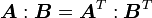 and using the
symmetry of , we have
and using the
symmetry of , we have
![\boldsymbol{S}:\dot{\boldsymbol{E}} =
\frac{1}{2}[(\boldsymbol{S}\cdot\boldsymbol{F}^T):\dot{\boldsymbol{F}}^T + (\boldsymbol{F}\cdot\boldsymbol{S}):\dot{\boldsymbol{F}}] =
\frac{1}{2}[(\boldsymbol{F}\cdot\boldsymbol{S}^T):\dot{\boldsymbol{F}} + (\boldsymbol{F}\cdot\boldsymbol{S}):\dot{\boldsymbol{F}}] =
(\boldsymbol{F}\cdot\boldsymbol{S}):\dot{\boldsymbol{F}} ~.](../I/m/c57b31cac2250472999481befab87360.png)
Now, 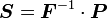 . Therefore,
 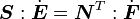 .
Hence, the stress power can be expressed as
.
Hence, the stress power can be expressed as
|
|
If we split the velocity gradient into symmetric and skew parts using
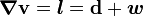
where  is the rate of deformation tensor and
  is the spin tensor,
we have
is the spin tensor,
we have

Since is symmetric and is skew, we have  .
Therefore,
.
Therefore,  . Hence, we may also
express the stress power as
. Hence, we may also
express the stress power as
|
|

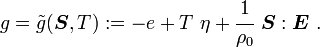
Helmholtz and Gibbs free energy
Recall that
Therefore,
Also recall that

Now, the internal energy  is a function only of the Green strain and the specific entropy. Let us assume, that the above relations can be uniquely inverted locally at a material point so that we have

Then the specific internal energy, the specific entropy, and the stress can also be expressed as functions of and , or and , i.e.,

We can show that

and

We define the Helmholtz free energy as
|
|
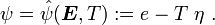
We define the Gibbs free energy as
|
|
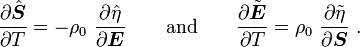
The functions  and
and  are unique. Using
these definitions it can be shown that
are unique. Using
these definitions it can be shown that

and
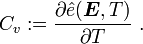
Specific Heats
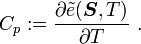
The specific heat at constant strain (or constant volume) is defined as
|
|
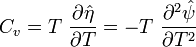
The specific heat at constant stress (or constant pressure) is defined as
|
|
We can show that
and
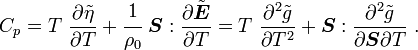
Also the equation for the balance of energy can be expressed in terms of the specific heats as
|
|
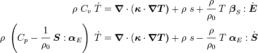
where
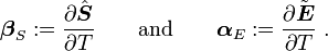
The quantity  is called the coefficient of thermal stress and the quantity
  is called the coefficient of thermal expansion.
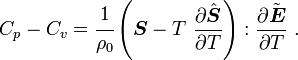
The difference between  and
and  can be expressed as
However, it is more common to express the above relation in terms of the elastic modulus tensor as
|
|
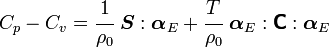
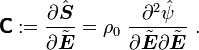
where the fourth-order tensor of elastic moduli is defined as
For isotropic materials with a constant coefficient of thermal expansion that follow the St. Venant-Kirchhoff material model, we can show that
![C_p - C_v = \cfrac{1}{\rho_0}\left[\alpha~\text{tr}{\boldsymbol{S}} +
9~\alpha^2~K~T\right]~.](../I/m/93df445060a8f71c313ad1165d48c97e.png)
References
- T. W. Wright. The Physics and Mathematics of Adiabatic Shear Bands. Cambridge University Press, Cambridge, UK, 2002.
- R. C. Batra. Elements of Continuum Mechanics. AIAA, Reston, VA., 2006.
- G. A. Maugin. The Thermomechanics of Nonlinear Irreversible Behaviors: An Introduction. World Scientific, Singapore, 1999.