Continuum mechanics/Thermodynamics of continua

Governing Equations

The equations that govern the thermomechanics of a solid include the balance laws for mass, momentum, and energy. Kinematic equations and constitutive relations are needed to complete the system of equations. Physical restrictions on the form of the constitutive relations are imposed by an entropy inequality that expresses the second law of thermodynamics in mathematical form.

The balance laws express the idea that the rate of change of a quantity (mass, momentum, energy) in a volume must arise from three causes:

the physical quantity itself flows through the surface that bounds the volume,
there is a source of the physical quantity on the surface of the volume, or/and,
there is a source of the physical quantity inside the volume.

Let $\Omega$ be the body (an open subset of Euclidean space) and let $\partial \Omega$ be its surface (the boundary of $\Omega$ ).

Let the motion of material points in the body be described by the map

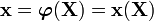
\mathbf{x} = \boldsymbol{\varphi}(\mathbf{X}) = \mathbf{x}(\mathbf{X})

where $\mathbf{X}$ is the position of a point in the initial configuration and $\mathbf{x}$ is the location of the same point in the deformed configuration.

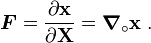
Recall that the deformation gradient ( $\boldsymbol{F}$ ) is given by

\boldsymbol{F} = \frac{\partial \mathbf{x}}{\partial \mathbf{X}} = \boldsymbol{\nabla}_{\circ} \mathbf{x} ~.

Balance Laws

Let $f(\mathbf{x},t)$ be a physical quantity that is flowing through the body. Let $g(\mathbf{x},t)$ be sources on the surface of the body and let $h(\mathbf{x},t)$ be sources inside the body. Let $\mathbf{n}(\mathbf{x},t)$ be the outward unit normal to the surface $\partial \Omega$ . Let $\mathbf{v}(\mathbf{x},t)$ be the velocity of the physical particles that carry the physical quantity that is flowing. Also, let the speed at which the bounding surface $\partial \Omega$ is moving be $u_n$ (in the direction $\mathbf{n}$ ).

Then, balance laws can be expressed in the general form

\cfrac{d}{dt}\left[\int_{\Omega} f(\mathbf{x},t)~\text{dV}\right] = \int_{\partial \Omega } f(\mathbf{x},t)[u_n(\mathbf{x},t) - \mathbf{v}(\mathbf{x},t)\cdot\mathbf{n}(\mathbf{x},t)]~\text{dA} + \int_{\partial \Omega } g(\mathbf{x},t)~\text{dA} + \int_{\Omega} h(\mathbf{x},t)~\text{dV} ~.

Note that the functions $f(\mathbf{x},t)$ , $g(\mathbf{x},t)$ , and $h(\mathbf{x},t)$ can be scalar valued, vector valued, or tensor valued - depending on the physical quantity that the balance equation deals with.

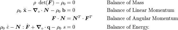
It can be shown that the balance laws of mass, momentum, and energy can be written as

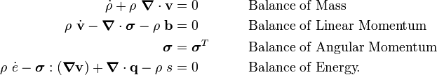
{ \begin{align} \dot{\rho} + \rho~\boldsymbol{\nabla} \cdot \mathbf{v} & = 0 & & \qquad\text{Balance of Mass} \\ \rho~\dot{\mathbf{v}} - \boldsymbol{\nabla} \cdot \boldsymbol{\sigma} - \rho~\mathbf{b} & = 0 & & \qquad\text{Balance of Linear Momentum} \\ \boldsymbol{\sigma} & = \boldsymbol{\sigma}^T & & \qquad\text{Balance of Angular Momentum} \\ \rho~\dot{e} - \boldsymbol{\sigma}:(\boldsymbol{\nabla}\mathbf{v}) + \boldsymbol{\nabla} \cdot \mathbf{q} - \rho~s & = 0 & & \qquad\text{Balance of Energy.} \end{align} }

In the above equations $\rho(\mathbf{x},t)$ is the mass density (current), $\dot{\rho}$ is the material time derivative of $\rho$ , $\mathbf{v}(\mathbf{x},t)$ is the particle velocity, $\dot{\mathbf{v}}$ is the material time derivative of $\mathbf{v}$ , $\boldsymbol{\sigma}(\mathbf{x},t)$ is the Cauchy stress tensor, $\mathbf{b}(\mathbf{x},t)$ is the body force density, $e(\mathbf{x},t)$ is the internal energy per unit mass, $\dot{e}$ is the material time derivative of $e$ , $\mathbf{q}(\mathbf{x},t)$ is the heat flux vector, and $s(\mathbf{x},t)$ is an energy source per unit mass.

With respect to the reference configuration, the balance laws can be written as

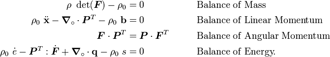
{ \begin{align} \rho~\det(\boldsymbol{F}) - \rho_0 &= 0 & & \qquad \text{Balance of Mass} \\ \rho_0~\ddot{\mathbf{x}} - \boldsymbol{\nabla}_{\circ}\cdot\boldsymbol{P}^T -\rho_0~\mathbf{b} & = 0 & & \qquad \text{Balance of Linear Momentum} \\ \boldsymbol{F}\cdot\boldsymbol{P}^T & = \boldsymbol{P}\cdot\boldsymbol{F}^T & & \qquad \text{Balance of Angular Momentum} \\ \rho_0~\dot{e} - \boldsymbol{P}^T:\dot{\boldsymbol{F}} + \boldsymbol{\nabla}_{\circ}\cdot\mathbf{q} - \rho_0~s & = 0 & & \qquad\text{Balance of Energy.} \end{align} }

In the above, $\boldsymbol{P}$ is the first Piola-Kirchhoff stress tensor, and $\rho_0$ is the mass density in the reference configuration. The first Piola-Kirchhoff stress tensor is related to the Cauchy stress tensor by

\boldsymbol{P} = J~\boldsymbol{\sigma}\cdot\boldsymbol{F}^{-T} ~\text{where}~ J = \det(\boldsymbol{F})

We can alternatively define the nominal stress tensor $\boldsymbol{N}$ which is the transpose of the first Piola-Kirchhoff stress tensor such that

\boldsymbol{N} = \boldsymbol{P}^T = J~\boldsymbol{F}^{-1}\cdot\boldsymbol{\sigma} ~.

Then the balance laws become

{ \begin{align} \rho~\det(\boldsymbol{F}) - \rho_0 &= 0 & & \qquad \text{Balance of Mass} \\ \rho_0~\ddot{\mathbf{x}} - \boldsymbol{\nabla}_{\circ}\cdot\boldsymbol{N} -\rho_0~\mathbf{b} & = 0 & & \qquad \text{Balance of Linear Momentum} \\ \boldsymbol{F}\cdot\boldsymbol{N} & = \boldsymbol{N}^T\cdot\boldsymbol{F}^T & & \qquad \text{Balance of Angular Momentum} \\ \rho_0~\dot{e} - \boldsymbol{N}:\dot{\boldsymbol{F}} + \boldsymbol{\nabla}_{\circ}\cdot\mathbf{q} - \rho_0~s & = 0 & & \qquad\text{Balance of Energy.} \end{align} }

Keep in mind that:

The gradient and divergence operators are defined such that

$\boldsymbol{\nabla} \mathbf{v} = \sum_{i,j = 1}^3 \frac{\partial v_i}{\partial x_j}\mathbf{e}_i\otimes\mathbf{e}_j = v_{i,j}\mathbf{e}_i\otimes\mathbf{e}_j ~;~~ \boldsymbol{\nabla} \cdot \mathbf{v} = \sum_{i=1}^3 \frac{\partial v_i}{\partial x_i} = v_{i,i} ~;~~ \boldsymbol{\nabla} \cdot \boldsymbol{S} = \sum_{i,j=1}^3 \frac{\partial S_{ij}}{\partial x_j}~\mathbf{e}_i = \sigma_{ij,j}~\mathbf{e}_i ~.$

where $\mathbf{v}$ is a vector field, $\boldsymbol{S}$ is a second-order tensor field, and $\mathbf{e}_i$ are the components of an orthonormal basis in the current configuration. Also,

$\boldsymbol{\nabla}_{\circ} \mathbf{v} = \sum_{i,j = 1}^3 \frac{\partial v_i}{\partial X_j}\mathbf{E}_i\otimes\mathbf{E}_j = v_{i,j}\mathbf{E}_i\otimes\mathbf{E}_j ~;~~ \boldsymbol{\nabla}_{\circ}\cdot\mathbf{v} = \sum_{i=1}^3 \frac{\partial v_i}{\partial X_i} = v_{i,i} ~;~~ \boldsymbol{\nabla}_{\circ}\cdot\boldsymbol{S} = \sum_{i,j=1}^3 \frac{\partial S_{ij}}{\partial X_j}~\mathbf{E}_i = S_{ij,j}~\mathbf{E}_i$

where $\mathbf{v}$ is a vector field, $\boldsymbol{S}$ is a second-order tensor field, and $\mathbf{E}_i$ are the components of an orthonormal basis in the reference configuration.

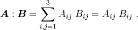
The inner product is defined as

$\boldsymbol{A}:\boldsymbol{B} = \sum_{i,j=1}^3 A_{ij}~B_{ij} = A_{ij}~B_{ij} ~.$

The Clausius-Duhem Inequality

The Clausius-Duhem inequality can be used to express the second law of thermodynamics for elastic-plastic materials. This inequality is a statement concerning the irreversibility of natural processes, especially when energy dissipation is involved.

Just like in the balance laws in the previous section, we assume that there is a flux of a quantity, a source of the quantity, and an internal density of the quantity per unit mass. The quantity of interest in this case is the entropy. Thus, we assume that there is an entropy flux, an entropy source, and an internal entropy density per unit mass ( $\eta$ ) in the region of interest.

Let $\Omega$ be such a region and let $\partial \Omega$ be its boundary. Then the second law of thermodynamics states that the rate of increase of $\eta$ in this region is greater than or equal to the sum of that supplied to $\Omega$ (as a flux or from internal sources) and the change of the internal entropy density due to material flowing in and out of the region.

Let $\partial \Omega$ move with a velocity $u_n$ and let particles inside $\Omega$ have velocities $\mathbf{v}$ . Let $\mathbf{n}$ be the unit outward normal to the surface $\partial \Omega$ . Let $\rho$ be the density of matter in the region, $\bar{q}$ be the entropy flux at the surface, and $r$ be the entropy source per unit mass. Then the entropy inequality may be written as

\cfrac{d}{dt}\left(\int_{\Omega} \rho~\eta~\text{dV}\right) \ge \int_{\partial \omega} \rho~\eta~(u_n - \mathbf{v}\cdot\mathbf{n})~\text{dA} + \int_{\partial \omega} \bar{q}~\text{dA} + \int_{\Omega} \rho~r~\text{dV} ~.

The scalar entropy flux can be related to the vector flux at the surface by the relation 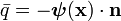$\bar{q} = -\boldsymbol{\psi}(\mathbf{x})\cdot\mathbf{n}$ . Under the assumption of incrementally isothermal conditions, we have

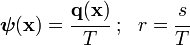
\boldsymbol{\psi}(\mathbf{x}) = \cfrac{\mathbf{q}(\mathbf{x})}{T} ~;~~ r = \cfrac{s}{T}

where $\mathbf{q}$ is the heat flux vector, $s$ is a energy source per unit mass, and $T$ is the absolute temperature of a material point at $\mathbf{x}$ at time $t$ .

We then have the Clausius-Duhem inequality in integral form:

{ \cfrac{d}{dt}\left(\int_{\Omega} \rho~\eta~\text{dV}\right) \ge \int_{\partial \omega} \rho~\eta~(u_n - \mathbf{v}\cdot\mathbf{n})~\text{dA} - \int_{\partial \omega} \cfrac{\mathbf{q}\cdot\mathbf{n}}{T}~\text{dA} + \int_{\Omega} \cfrac{\rho~s}{T}~\text{dV} ~. }

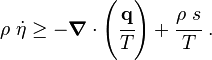
We can show that the entropy inequality may be written in differential form as

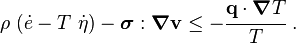
{ \rho~\dot{\eta} \ge - \boldsymbol{\nabla} \cdot \left(\cfrac{\mathbf{q}}{T}\right) + \cfrac{\rho~s}{T} ~. }

In terms of the Cauchy stress and the internal energy, the Clausius-Duhem inequality may be written as

Clausius-Duhem inequality

{ \rho~(\dot{e} - T~\dot{\eta}) - \boldsymbol{\sigma}:\boldsymbol{\nabla}\mathbf{v} \le - \cfrac{\mathbf{q}\cdot\boldsymbol{\nabla} T}{T} ~. }

References

T. W. Wright. (2002) The Physics and Mathematics of Adiabatic Shear Bands. Cambridge University Press, Cambridge, UK.
R. C. Batra. (2006) Elements of Continuum Mechanics. AIAA, Reston, VA.
G. A. Maugin. (1999) The Thermomechanics of Nonlinear Irreversible Behaviors: An Introduction. World Scientific, Singapore.
M. E. Gurtin. (1981) An Introduction to Continuum Mechanics. Academic Press, New York.

This article is issued from Wikiversity - version of the Saturday, May 10, 2008. The text is available under the Creative Commons Attribution/Share Alike but additional terms may apply for the media files.