Continuum mechanics/Spectral decomposition

Spectral decompositions

Many numerical algorithms use spectral decompositions to compute material behavior.

Spectral decompositions of stretch tensors

Infinitesimal line segments in the material and spatial configurations are related by

d\mathbf{x} = \boldsymbol{F}\cdot d\boldsymbol{X} = \boldsymbol{R}\cdot(\boldsymbol{U} \cdot d\boldsymbol{X}) = \boldsymbol{V} \cdot (\boldsymbol{R} \cdot d\boldsymbol{X}) ~.

So the sequence of operations may be either considered as a stretch of in the material configuration followed by a rotation or a rotation followed by a stretch.

Also note that

\boldsymbol{V} = \boldsymbol{R}\cdot\boldsymbol{U}\cdot\boldsymbol{R}^T ~.

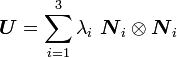
Let the spectral decomposition of $\boldsymbol{U}$ be

\boldsymbol{U} = \sum_{i=1}^3 \lambda_i~\boldsymbol{N}_i\otimes\boldsymbol{N}_i

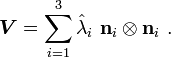
and the spectral decomposition of $\boldsymbol{V}$ be

\boldsymbol{V} = \sum_{i=1}^3 \hat{\lambda}_i~\mathbf{n}_i\otimes\mathbf{n}_i ~.

Then

\boldsymbol{V} = \boldsymbol{R}\cdot\boldsymbol{U}\cdot\boldsymbol{R}^T = \sum_{i=1}^3 \lambda_i~\boldsymbol{R}\cdot(\boldsymbol{N}_i\otimes\boldsymbol{N}_i)\cdot\boldsymbol{R}^T = \sum_{i=1}^3 \lambda_i~(\boldsymbol{R}\cdot\boldsymbol{N}_i)\otimes(\boldsymbol{R}\cdot\boldsymbol{N}_i)

Therefore the uniqueness of the spectral decomposition implies that

\lambda_i = \hat{\lambda}_i \quad \text{and} \quad \mathbf{n}_i = \boldsymbol{R}\cdot\boldsymbol{N}_i

The left stretch ( $\boldsymbol{V}$ ) is also called the spatial stretch tensor while the right stretch ( $\boldsymbol{U}$ ) is called the material stretch tensor.

Spectral decompositions of deformation gradient

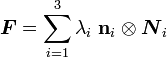
The deformation gradient is given by

\boldsymbol{F} = \boldsymbol{R}\cdot\boldsymbol{U}

In terms of the spectral decomposition of $\boldsymbol{U}$ we have

\boldsymbol{F} = \sum_{i=1}^3 \lambda_i~\boldsymbol{R}\cdot(\boldsymbol{N}_i\otimes\boldsymbol{N}_i) = \sum_{i=1}^3 \lambda_i~(\boldsymbol{R}\cdot\boldsymbol{N}_i)\otimes\boldsymbol{N}_i = \sum_{i=1}^3 \lambda_i~\mathbf{n}_i\otimes\boldsymbol{N}_i

Therefore the spectral decomposition of $\boldsymbol{F}$ can be written as

\boldsymbol{F} = \sum_{i=1}^3 \lambda_i~\mathbf{n}_i\otimes\boldsymbol{N}_i

Let us now see what effect the deformation gradient has when it is applied to the eigenvector $\boldsymbol{N}_i$ .

We have

\boldsymbol{F}\cdot\boldsymbol{N}_i = \boldsymbol{R}\cdot\boldsymbol{U}\cdot\boldsymbol{N}_i = \boldsymbol{R}\cdot\left(\sum_{j=1}^3 \lambda_j~\boldsymbol{N}_j\otimes\boldsymbol{N}_j\right)\cdot \boldsymbol{N}_i

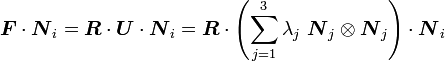
From the definition of the dyadic product

(\mathbf{u}\otimes\mathbf{v})\cdot\mathbf{w} = (\mathbf{w}\cdot\mathbf{v})~\mathbf{u}

Since the eigenvectors are orthonormal, we have

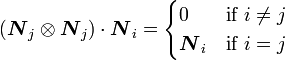
(\boldsymbol{N}_j\otimes\boldsymbol{N}_j)\cdot\boldsymbol{N}_i = \begin{cases} 0 & \mbox{if}~ i \ne j \\ \boldsymbol{N}_i & \mbox{if}~ i = j \end{cases}

Therefore,

\left(\sum_{j=1}^3 \lambda_j~\boldsymbol{N}_j\otimes\boldsymbol{N}_j\right)\cdot \boldsymbol{N}_i = \lambda_i~\boldsymbol{N}_i \text{no sum on}~i

That leads to

\boldsymbol{F}\cdot\boldsymbol{N}_i = \lambda_i~(\boldsymbol{R}\cdot\boldsymbol{N}_i) = \lambda_i~\mathbf{n}_i

So the effect of $\boldsymbol{F}$ on $\boldsymbol{N}_i$ is to stretch the vector by $\lambda_i$ and to rotate it to the new orientation $\mathbf{n}_i$ .

We can also show that

\boldsymbol{F}^{-T}\cdot\boldsymbol{N}_i = \cfrac{1}{\lambda_i}~\mathbf{n}_i ~;~~ \boldsymbol{F}^T\cdot\mathbf{n}_i = \lambda_i~\boldsymbol{N}_i ~;~~ \boldsymbol{F}^{-1}\cdot\mathbf{n}_i = \cfrac{1}{\lambda_i}~\boldsymbol{N}_i

Spectral decompositions of strains

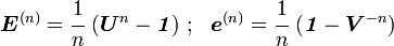
Recall that the Lagrangian Green strain and its Eulerian counterpart are defined as

\boldsymbol{E} = \frac{1}{2}~(\boldsymbol{F}^T\cdot\boldsymbol{F} - \boldsymbol{\mathit{1}}) ~;~~ \boldsymbol{e} = \frac{1}{2}~(\boldsymbol{\mathit{1}} - \left(\boldsymbol{F}\cdot\boldsymbol{F}^T\right)^{-1})

Now,

\boldsymbol{F}^T\cdot\boldsymbol{F} = \boldsymbol{U}\cdot\boldsymbol{R}^T\cdot\boldsymbol{R}\cdot\boldsymbol{U} = \boldsymbol{U}^2 ~;~~ \boldsymbol{F}\cdot\boldsymbol{F}^T = \boldsymbol{V}\cdot\boldsymbol{R}\cdot\boldsymbol{R}^T\cdot\boldsymbol{V} = \boldsymbol{V}^2

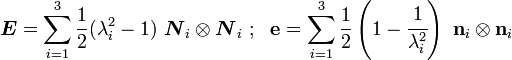
Therefore we can write

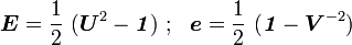
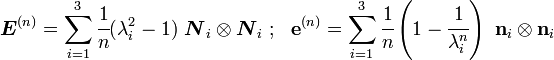
\boldsymbol{E} = \frac{1}{2}~(\boldsymbol{U}^2 - \boldsymbol{\mathit{1}}) ~;~~ \boldsymbol{e} = \frac{1}{2}~(\boldsymbol{\mathit{1}} - \boldsymbol{V}^{-2})

Hence the spectral decompositions of these strain tensors are

\boldsymbol{E} = \sum_{i=1}^3 \frac{1}{2}(\lambda_i^2 - 1)~\boldsymbol{N}_i\otimes\boldsymbol{N}_i ~;~~ \mathbf{e} = \sum_{i=1}^3 \frac{1}{2}\left(1 - \cfrac{1}{\lambda_i^2}\right)~ \mathbf{n}_i\otimes\mathbf{n}_i

Generalized strain measures

We can generalize these strain measures by defining strains as

\boldsymbol{E}^{(n)} = \cfrac{1}{n}~(\boldsymbol{U}^n - \boldsymbol{\mathit{1}}) ~;~~ \boldsymbol{e}^{(n)} = \cfrac{1}{n}~(\boldsymbol{\mathit{1}} - \boldsymbol{V}^{-n})

The spectral decomposition is

\boldsymbol{E}^{(n)} = \sum_{i=1}^3 \cfrac{1}{n}(\lambda_i^2 - 1)~\boldsymbol{N}_i\otimes\boldsymbol{N}_i ~;~~ \mathbf{e}^{(n)} = \sum_{i=1}^3 \cfrac{1}{n}\left(1 - \cfrac{1}{\lambda_i^n}\right)~ \mathbf{n}_i\otimes\mathbf{n}_i

Clearly, the usual Green strains are obtained when $n=2$ .

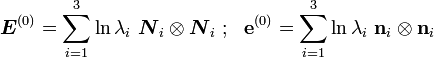
Logarithmic strain measure

A strain measure that is commonly used is the logarithmic strain measure. This strain measure is obtained when we have $n \rightarrow 0$ . Thus

\boldsymbol{E}^{(0)} = \ln(\boldsymbol{U}) ~;~~ \boldsymbol{e}^{(0)} = \ln(\boldsymbol{V})

The spectral decomposition is

\boldsymbol{E}^{(0)} = \sum_{i=1}^3 \ln\lambda_i~\boldsymbol{N}_i\otimes\boldsymbol{N}_i ~;~~ \mathbf{e}^{(0)} = \sum_{i=1}^3 \ln\lambda_i~\mathbf{n}_i\otimes\mathbf{n}_i

This article is issued from Wikiversity - version of the Tuesday, August 28, 2007. The text is available under the Creative Commons Attribution/Share Alike but additional terms may apply for the media files.