Continuum mechanics/Nonlinear elasticity
< Continuum mechanicsThere are two types models of nonlinear elastic behavior that are in common use. These are :
- Hyperelasticity
- Hypoelasticity
Hyperelasticity
Hyperelastic materials are truly elastic in the sense that if a load is applied to such a material and then removed, the material returns to its original shape without any dissipation of energy in the process. In other word, a hyperelastic material stores energy during loading and releases exactly the same amount of energy during unloading. There is no path dependence.
If  is the Helmholtz free energy, then the stress-strain behavior for such a material is given by
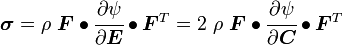
where  is the Cauchy stress,
  is the current mass density,
  is the deformation gradient,
  is the Lagrangian Green strain tensor, and
  is the left Cauchy-Green deformation tensor.
We can use the relationship between the Cauchy stress and the 2nd Piola-Kirchhoff stress to obtain an alternative relation between stress and strain.
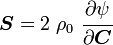
where  is the 2nd Piola-Kirchhoff stress and
  is the mass density in the reference configuration.
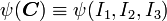
Isotropic hyperelasticity
For isotropic materials, the free energy must be an isotropic function of . This also mean that the free energy must depend only on the principal invariants of which are
![\begin{align}
I_{\boldsymbol{C}} = I_1 & = \text{tr}(\mathbf{C}) = C_{ii} = \lambda_1^2 + \lambda_2^2 + \lambda_3^2 \\
II_{\boldsymbol{C}} = I_2 & = \tfrac{1}{2}\left[\text{tr}(\mathbf{C}^2) - (\text{tr}~\mathbf{C})^2 \right]
= \tfrac{1}{2}\left[C_{ik}C_{ki} - C_{jj}^2\right] = \lambda_1^2\lambda_2^2 + \lambda_2^2\lambda_3^2 + \lambda_3^2\lambda_1^2 \\
III_{\boldsymbol{C}} = I_3 & = \det(\mathbf{C}) = \lambda_1^2\lambda_2^2\lambda_3^2
\end{align}](../I/m/9c485f28608801c922f15878e3c8f077.png)
In other words,
Therefore, from the chain rule,

From the Cayley-Hamilton theorem we can show that

Hence we can also write
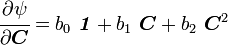
The stress-strain relation can then be written as
![\boldsymbol{S} = 2~\rho_0~\left[b_0~\boldsymbol{\mathit{1}} + b_1~\boldsymbol{C} + b_2~\boldsymbol{C}^2\right]](../I/m/9c9d97220df7cf84a4af3071bfd5e4eb.png)
A similar relation can be obtained for the Cauchy stress which has the form
![\boldsymbol{\sigma} = 2~\rho~\left[a_2~\boldsymbol{\mathit{1}} + a_0~\boldsymbol{B} + a_1~\boldsymbol{B}^2\right]](../I/m/b81f4e067f6c6b2de748a0433e34780d.png)
where  is the right Cauchy-Green deformation tensor.
Cauchy stress in terms of invariants
For w:isotropic hyperelastic materials, the Cauchy stress can be expressed in terms of the invariants of the left Cauchy-Green deformation tensor (or right Cauchy-Green deformation tensor). If the w:strain energy density function is  , then
![\begin{align}
\boldsymbol{\sigma} & =
\cfrac{2}{\sqrt{I_3}}\left[\left(\cfrac{\partial\hat{W}}{\partial I_1} + I_1~\cfrac{\partial\hat{W}}{\partial I_2}\right)\boldsymbol{B} - \cfrac{\partial\hat{W}}{\partial I_2}~\boldsymbol{B} \cdot\boldsymbol{B} \right] + 2\sqrt{I_3}~\cfrac{\partial\hat{W}}{\partial I_3}~\boldsymbol{\mathit{1}} \\
& = \cfrac{2}{J}\left[\cfrac{1}{J^{2/3}}\left(\cfrac{\partial\bar{W}}{\partial \bar{I}_1} + \bar{I}_1~\cfrac{\partial\bar{W}}{\partial \bar{I}_2}\right)\boldsymbol{B} -
\cfrac{1}{3}\left(\bar{I}_1~\cfrac{\partial\bar{W}}{\partial \bar{I}_1} + 2~\bar{I}_2~\cfrac{\partial\bar{W}}{\partial \bar{I}_2}\right)\boldsymbol{\mathit{1}} - \right.\\
& \qquad \qquad \qquad \left. \cfrac{1}{J^{4/3}}~\cfrac{\partial\bar{W}}{\partial \bar{I}_2}~\boldsymbol{B} \cdot\boldsymbol{B} \right] + \cfrac{\partial\bar{W}}{\partial J}~\boldsymbol{\mathit{1}} \\
& = \cfrac{\lambda_1}{\lambda_1\lambda_2\lambda_3}~\cfrac{\partial\tilde{W}}{\partial \lambda_1}~\mathbf{n}_1\otimes\mathbf{n}_1 + \cfrac{\lambda_2}{\lambda_1\lambda_2\lambda_3}~\cfrac{\partial\tilde{W}}{\partial \lambda_2}~\mathbf{n}_2\otimes\mathbf{n}_2 + \cfrac{\lambda_3}{\lambda_1\lambda_2\lambda_3}~\cfrac{\partial\tilde{W}}{\partial \lambda_3}~\mathbf{n}_3\otimes\mathbf{n}_3
\end{align}](../I/m/67a20501d39e70137edf2eb8a24e28de.png)
(See the page on the left Cauchy-Green deformation tensor for the definitions of these symbols).
Proof 1: The second Piola-Kirchhoff stress tensor for a hyperelastic material is given by where
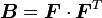
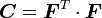 is the right Cauchy-Green deformation tensor and is the deformation gradient. The Cauchy stress is given by
where
 . Let
. Let  be the three principal invariants of . Then
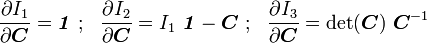
The derivatives of the invariants of the symmetric tensor
areTherefore we can write
Plugging into the expression for the Cauchy stress gives
Using the left Cauchy-Green deformation tensor
 and noting that
  , we can write
Proof 2: To express the Cauchy stress in terms of the invariants  recall that
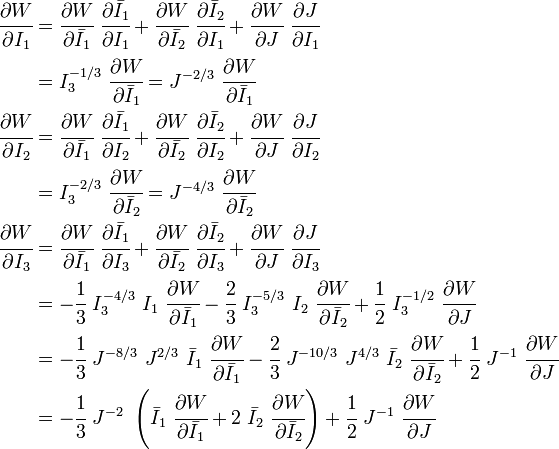
The chain rule of differentiation gives us
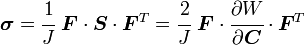
Recall that the Cauchy stress is given by
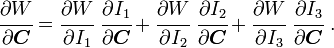
In terms of the invariants
we havePlugging in the expressions for the derivatives of
 in terms of , we have
or,
Proof 3: To express the Cauchy stress in terms of the stretches  recall that
The chain rule gives
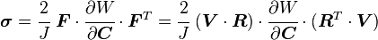
The Cauchy stress is given by
Plugging in the expression for the derivative of
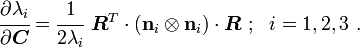
leads toUsing the spectral decomposition of
 we have
Also note that
Therefore the expression for the Cauchy stress can be written as


![\boldsymbol{\sigma}
= \cfrac{2}{J}~\left[\cfrac{\partial W}{\partial I_1}~\boldsymbol{F}\cdot\boldsymbol{F}^T+
\cfrac{\partial W}{\partial I_2}~(I_1~\boldsymbol{F}\cdot\boldsymbol{F}^T - \boldsymbol{F}\cdot\boldsymbol{F}^T\cdot\boldsymbol{F}\cdot\boldsymbol{F}^T) +
\cfrac{\partial W}{\partial I_3}~I_3~\boldsymbol{\mathit{1}}\right]](../I/m/d91ec0d967022cfc301c91b9bcd58c7b.png)
![\boldsymbol{\sigma}
= \cfrac{2}{\sqrt{I_3}}~\left[\left(\cfrac{\partial W}{\partial I_1} +
I_1~\cfrac{\partial W}{\partial I_2}\right)~\boldsymbol{B} -
\cfrac{\partial W}{\partial I_2}~\boldsymbol{B}\cdot\boldsymbol{B}\right] +
2~\sqrt{I_3}~\cfrac{\partial W}{\partial I_3}~\boldsymbol{\mathit{1}}~.](../I/m/bdd414d8607559f38a725e128ad07a42.png)

![\boldsymbol{\sigma}
= \cfrac{2}{J}~\left[\left(\cfrac{\partial W}{\partial I_1}+
J^{2/3}~\bar{I}_1~\cfrac{\partial W}{\partial I_2}\right)~\boldsymbol{B} -
\cfrac{\partial W}{\partial I_2}~\boldsymbol{B}\cdot\boldsymbol{B}\right] +
2~J~\cfrac{\partial W}{\partial I_3}~\boldsymbol{\mathit{1}}~.](../I/m/00f40ca07d5b1ccece93577174a4151e.png)
![\begin{align}
\boldsymbol{\sigma}
& = \cfrac{2}{J}~\left[\left(J^{-2/3}~\cfrac{\partial W}{\partial \bar{I}_1} +
J^{-2/3}~\bar{I}_1~\cfrac{\partial W}{\partial \bar{I}_2}\right)~\boldsymbol{B} -
J^{-4/3}~\cfrac{\partial W}{\partial \bar{I}_2}~\boldsymbol{B}\cdot\boldsymbol{B}\right]
+ \\
& \qquad
2~J~\left[-\cfrac{1}{3}~J^{-2}~\left(\bar{I}_1~\cfrac{\partial W}{\partial \bar{I}_1}+
2~\bar{I}_2~\cfrac{\partial W}{\partial \bar{I}_2}\right) +
\cfrac{1}{2}~J^{-1}~\cfrac{\partial W}{\partial J}\right]~\boldsymbol{\mathit{1}}
\end{align}](../I/m/79c6b49b7d97914ba64863996d9a7221.png)
![\begin{align}
\boldsymbol{\sigma}
& = \cfrac{2}{J}~\left[\cfrac{1}{J^{2/3}}~\left(\cfrac{\partial W}{\partial \bar{I}_1} +
\bar{I}_1~\cfrac{\partial W}{\partial \bar{I}_2}\right)~\boldsymbol{B} -
\cfrac{1}{3}\left(\bar{I}_1~\cfrac{\partial W}{\partial \bar{I}_1}+
2~\bar{I}_2~\cfrac{\partial W}{\partial \bar{I}_2}\right)\boldsymbol{\mathit{1}} - \right. \\
& \qquad \left. \cfrac{1}{J^{4/3}}~
\cfrac{\partial W}{\partial \bar{I}_2}~\boldsymbol{B}\cdot\boldsymbol{B}\right]
+ \cfrac{\partial W}{\partial J}~\boldsymbol{\mathit{1}}
\end{align}](../I/m/f43da6a703b195491f296e9a1abf4e97.png)
![\begin{align}
\cfrac{\partial W}{\partial\boldsymbol{C}} & =
\cfrac{\partial W}{\partial \lambda_1}~\cfrac{\partial \lambda_1}{\partial\boldsymbol{C}} +
\cfrac{\partial W}{\partial \lambda_2}~\cfrac{\partial \lambda_2}{\partial\boldsymbol{C}} +
\cfrac{\partial W}{\partial \lambda_3}~\cfrac{\partial \lambda_3}{\partial\boldsymbol{C}} \\
& = \boldsymbol{R}^T\cdot\left[\cfrac{1}{2\lambda_1}~\cfrac{\partial W}{\partial \lambda_1}~\mathbf{n}_1\otimes\mathbf{n}_1 +
\cfrac{1}{2\lambda_2}~\cfrac{\partial W}{\partial \lambda_2}~\mathbf{n}_2\otimes\mathbf{n}_2 +
\cfrac{1}{2\lambda_3}~\cfrac{\partial W}{\partial \lambda_3}~\mathbf{n}_3\otimes\mathbf{n}_3\right]\cdot\boldsymbol{R}
\end{align}](../I/m/0690cc4f1466f2a40621280ac1f83ce6.png)
![\boldsymbol{\sigma} =
\cfrac{2}{J}~\boldsymbol{V}\cdot
\left[\cfrac{1}{2\lambda_1}~
\cfrac{\partial W}{\partial \lambda_1}~\mathbf{n}_1\otimes\mathbf{n}_1 +
\cfrac{1}{2\lambda_2}~
\cfrac{\partial W}{\partial \lambda_2}~\mathbf{n}_2\otimes\mathbf{n}_2 +
\cfrac{1}{2\lambda_3}~
\cfrac{\partial W}{\partial \lambda_3}~\mathbf{n}_3\otimes\mathbf{n}_3\right]
\cdot\boldsymbol{V}](../I/m/e16c3b5ec1b5bf612e7f244b105bed9e.png)


![\boldsymbol{\sigma} =
\cfrac{1}{\lambda_1\lambda_2\lambda_3}~
\left[\lambda_1~\cfrac{\partial W}{\partial \lambda_1}~\mathbf{n}_1\otimes\mathbf{n}_1 +
\lambda_2~\cfrac{\partial W}{\partial \lambda_2}~\mathbf{n}_2\otimes\mathbf{n}_2 +
\lambda_3~\cfrac{\partial W}{\partial \lambda_3}~\mathbf{n}_3\otimes\mathbf{n}_3
\right]](../I/m/8446943129c7cccf8ff25621e4ffdeac.png)
Saint-Venant–Kirchhoff material
The simplest constitutive relationship that satisfies the requirements of hyperelasticity is the Saint-Venant–Kirchhoff material, which has a response function of the form
where  and
and  are material constants that have to be determined by experiments. Such a linear relation is physically possible only for small strains.