Continuum mechanics/Motion and displacement

Continuum Mechanics

To understand the updated Lagrangian formulation and nonlinear finite elements of solids, we have to know continuum mechanics. A brief introduction to continuum mechanics is given in the following. If you find this handout difficult to follow, please read Chapter 2 from Belytschko's book and Chapter 9 from Reddy's book. You should also read an introductory text on continuum mechanics such as Nonlinear continuum mechanics for finite element analysis by Bonet and Wood.

Motion

Let the undeformed (or reference) configuration of the body be $\Omega_0$ and let the undeformed boundary be $\Gamma_0$ . Let the deformed (or current) configuration be $\Omega$ with boundary $\Gamma$ . Let $\boldsymbol{\varphi}(\mathbf{X},t)$ be the motion that takes the body from the reference to the current configuration (see Figure 1).

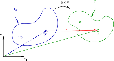Figure 1. The motion of a body.

We write

\mathbf{x} = \boldsymbol{\varphi}(\boldsymbol{X}, t)

where $\mathbf{x}$ is the position of material point $\boldsymbol{X}$ at time $t$ .

In index notation,

x_i = \varphi_i(X_j, t)~, \qquad i,j=1,2,3.

Displacement

The displacement of a material point is given by

\mathbf{u}(\boldsymbol{X},t) = \boldsymbol{\varphi}(\boldsymbol{X},t) - \boldsymbol{\varphi}(\boldsymbol{X},0) = \boldsymbol{\varphi}(\boldsymbol{X},t) - \boldsymbol{X}= \mathbf{x} - \boldsymbol{X}~.

In index notation,

u_i = \varphi_i(X_j, t) - X_j {\delta}_{ij}= x_i - X_j {\delta}_{ij} ~.

where ${\delta}_{ij}$ is the Kronecker delta.

Velocity

The velocity is the material time derivative of the motion (i.e., the time derivative with $\mathbf{X}$ held constant). This type of derivative is also called the total derivative.

\mathbf{v}(\boldsymbol{X}, t) = \frac{\partial }{\partial t}\left[\boldsymbol{\varphi}(\boldsymbol{X}, t)\right] ~.

Now,

\mathbf{u}(\boldsymbol{X},t) = \boldsymbol{\varphi}(\boldsymbol{X},t) - \boldsymbol{X} ~.

Therefore, the material time derivative of $\mathbf{u}$ is

\dot{\mathbf{u}} = \frac{\partial }{\partial t}\left[\mathbf{u}(\boldsymbol{X},t)\right] = \frac{\partial }{\partial t}\left[\boldsymbol{\varphi}(\boldsymbol{X},t) - \boldsymbol{X}\right] = \frac{\partial }{\partial t}\left[\boldsymbol{\varphi}(\boldsymbol{X},t)\right] = \mathbf{v}(\boldsymbol{X}, t) ~.

Alternatively, we could have expressed the velocity in terms of the spatial coordinates $\mathbf{x}$ . Let

\mathbf{u}(\mathbf{x}, t) = \mathbf{u}(\boldsymbol{\varphi}(\boldsymbol{X},t), t) ~.

Then the material time derivative of $\mathbf{u}(\mathbf{x},t)$ is

\cfrac{D}{Dt}\left[\mathbf{u}(\mathbf{x}, t)\right] = \frac{\partial \mathbf{u}}{\partial t} + \frac{\partial \mathbf{u}}{\partial \mathbf{x}}\frac{\partial \mathbf{x}}{\partial t} = \frac{\partial \mathbf{u}}{\partial t} + \frac{\partial \mathbf{u}}{\partial \mathbf{x}}\frac{\partial }{\partial t} \left[\boldsymbol{\varphi}(\boldsymbol{X},t)\right] = \mathbf{v}(\mathbf{x},t) + \frac{\partial \mathbf{u}}{\partial \mathbf{x}}\mathbf{v}(\boldsymbol{X},t) ~.

Acceleration

The acceleration is the material time derivative of the velocity of a material point.

\mathbf{a}(\boldsymbol{X}, t) = \frac{\partial }{\partial t}\left[\mathbf{v}(\boldsymbol{X}, t)\right] = \dot{\mathbf{v}} = \frac{\partial^2 }{\partial t^2}\left[\mathbf{u}(\boldsymbol{X},t)\right] = \ddot{\mathbf{u}} ~.

This article is issued from Wikiversity - version of the Tuesday, August 28, 2007. The text is available under the Creative Commons Attribution/Share Alike but additional terms may apply for the media files.